Frequentist statistical methods, despite their flaws, are generally serviceable for a large suite of practical problems faced by engineers during product development of medical devices. But even in domains where simple models usually do the trick, there remain instances where a Bayesian approach is the best (and perhaps only logical) way to tackle a problem.
In the rest of this post, I will lay out a technical use-case and associated modeling workflow that is based on a real business problem encountered in the medical device industry. Note: specifics have been changed to respect the privacy of the company and the product. Here we go.
Libraries
library(tidyverse)
library(gt)
library(tidybayes)
Background
The problem background is this:
Vascular implants like stents and heart valves are tested extensively on the bench prior to approval for clinical use. When fractures (failures) occur, it is the job of the engineering team to determine if the failure was due to the design of the implant itself or a special cause and also assess the potential risk to the patient.
Assume that we have observed an unanticipated fracture late in the design process - during the 3rd of 3 planned rounds of testing.
An investigation is unable to identify a special cause beyond the design of the implant. Management therefore wishes the understand the risk of a harm occurring in a patient implanted with this product based solely on the test data available, plus any additional information that may help inform the analysis, assuming no special cause for the fracture.
The probability of a patient harm occurring due to a fracture can be broken down into two components as follows:1
\[\mbox P_1 = \mbox{Probability of Fracture Occurring}\\\mbox P_2 = \mbox{Probability of Fracture Leading to a Harm}\]
Assuming independence, the probability of harm from the fracture is then:
\[\mbox P_h = \mathrm{P}(P_1 \cap P_2) = \mbox P_1 \mbox{ x }\mbox P_2\]
Our challenge is: how to develop an estimate of \(\mbox P_1 \mbox{ , }\mbox P_2 \mbox{ , and }\mbox P_h\) that incorporates the benchtop test data and our domain knowledge while also propagating uncertainty throughout the calculation.2
First, lets see what data and information we have available. Assume the following benchtop data and/or computer simulation (FEA) data are available to inform each estimate:
Analysis
Data for Probability of Fracture Occurring (P1)
To estimate \(\mbox P_1\) we have 3 rounds of benchtop data, where each outcome is a pass/fail representing fracture or no fracture.
- Round 1: 6 parts tested and all 6 passed (0 failures)
- Round 2: 5 parts tested and all 5 passed (0 failures)
- Round 3: 12 parts tested and 11 passed (1 failure). This is the failure that triggered the investigation.
Data for Probability of Fracture Leading to Harm (P2)
To simplify the problem, we’ll only consider one patient harm: embolism due to broken pieces of the implant migrating within the body. In order for this to happen, the first fracture (as observed on the bench in part 1, round 3) must cascade into additional fractures and eventual loss of overall implant integrity. In order to assess this \(\mbox P_2\) risk, we have 2 inputs:
- Input 1: A finite element analysis (FEA) simulation concluding that when 1 fracture occurs, the strain levels at other locations in the implant are not expected to rise to levels where we would anticipate additional fractures and loss of overall implant integrity
- Input 2: A benchtop study in which 6 parts were intentionally fractured at the location of interest continued to cycle; none of the 6 showed any additional fractures after the first (0 failures)
Note: FEA is a way to simulate stresses and strain in a model under specific assumptions of boundary conditions, geometries, material properties, etc. See below for an example of predicted strain amplitudes in a nitinol component via FEA.3

Modeling
We want a model that can use all the available information which includes several rounds of benchtop data and a computer simulation. A beta-binomial Bayesian model is a reasonable choice for both technical and business reasons, a few of which are shown below:4
- The model is simple, with an analytic solution available (to avoid needing to validate an MCMC sampler and supporting code)
- There is domain knowledge (FEA moel) available that needs to be incorporated into the analysis
- The outcome can be easily understood by a general audience
To generate the posterior probabilities for \(\mbox P_1\) we need nothing more than addition. The two parameters in the model are the cumulative sum of the 1+passes and 1+fails, respectively.
\[\mbox P_1 \sim \mbox{Beta}(\alpha_0+\mbox{fails}, \beta_0+\mbox{passes})\]
Model for P1
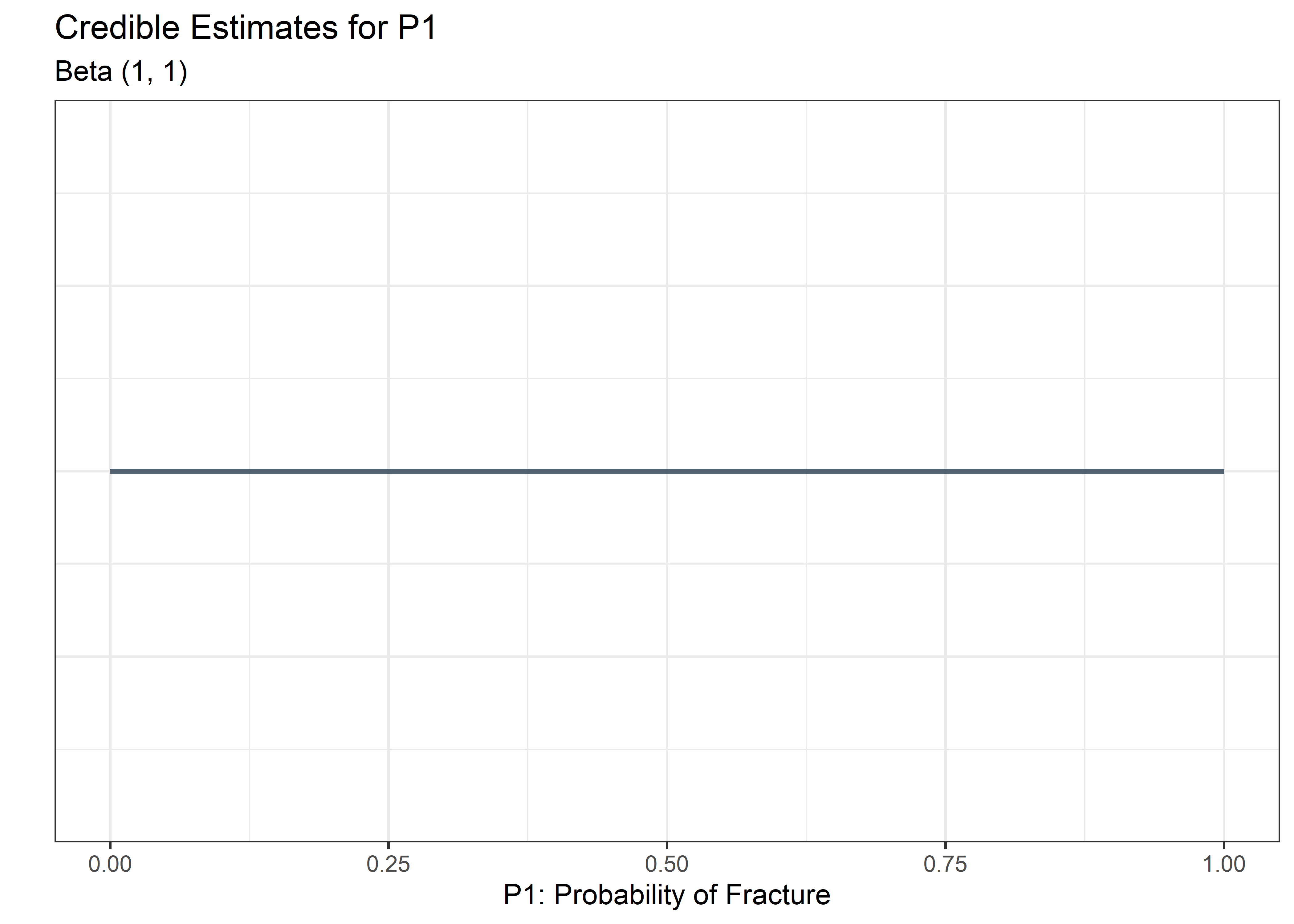
For \(\mbox P_1\) we can choose to start with a flat prior where \(\alpha_0\) and \(\beta_0\) are 1. This implies we don’t know anything about whether or not the part may fracture.
Before Seeing Data
p_1 <- tibble(x_canvas = c(0, 1))

alpha <- 1
beta <- 1

plot_p1_fcn <- function(a, b) {
  p_1 %>%
    ggplot(aes(x = x_canvas)) +
    stat_function(
      fun = dbeta,
      args = list(a, b),
      color = "#2c3e50",
      size = 1,
      alpha = .8
    ) +
    #  ylim(c(0, 1.5)) +
    labs(
      y = "",
      x = "P1: Probability of Fracture",
      title = "Credible Estimates for P1",
      subtitle = str_glue("Beta ({a}, {b})")
    ) +
    theme_bw() +
    theme(
      axis.text.y = element_blank(),
      axis.ticks.y = element_blank()
    )
}

plot_p1_fcn(a = alpha, b = beta)
Add Round 1 Benchtop Data
Recall from above:
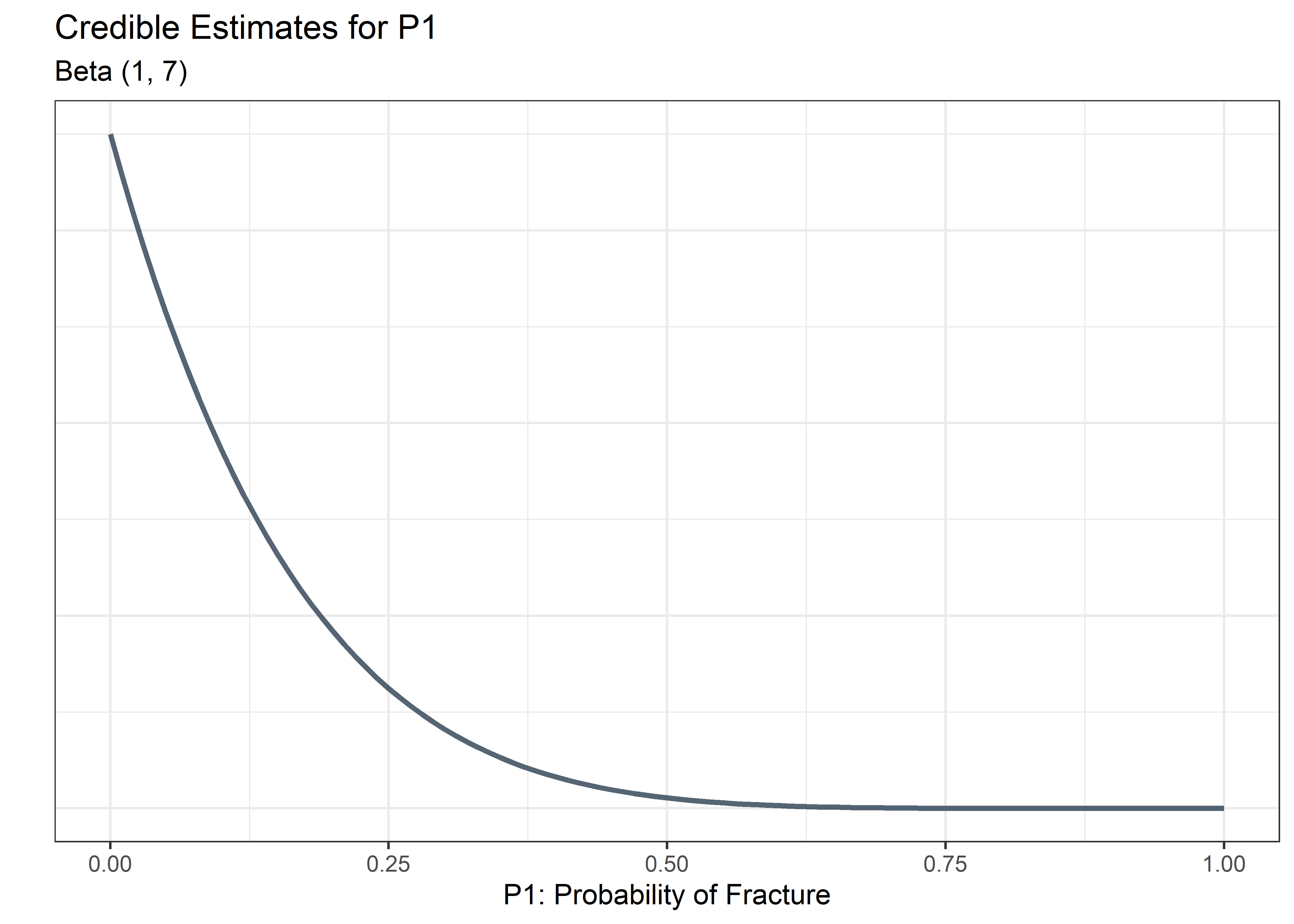
Round 1: 6 parts tested and all 6 passed (0 failures). So we add 6 to the cumulative sum for b and nothing to a.
alpha <- 1
beta <- 7

plot_p1_fcn(a = alpha, b = beta)
Add Round 2 Benchtop Data
Recall from above:
Round 2: 5 parts tested and all 5 passed (0 failures). So we add 5 to the cumulative sum for b and nothing to a.
alpha <- 1
beta <- 12

plot_p1_fcn(a = alpha, b = beta)
Add Round 3 Benchtop Data
Recall from above:
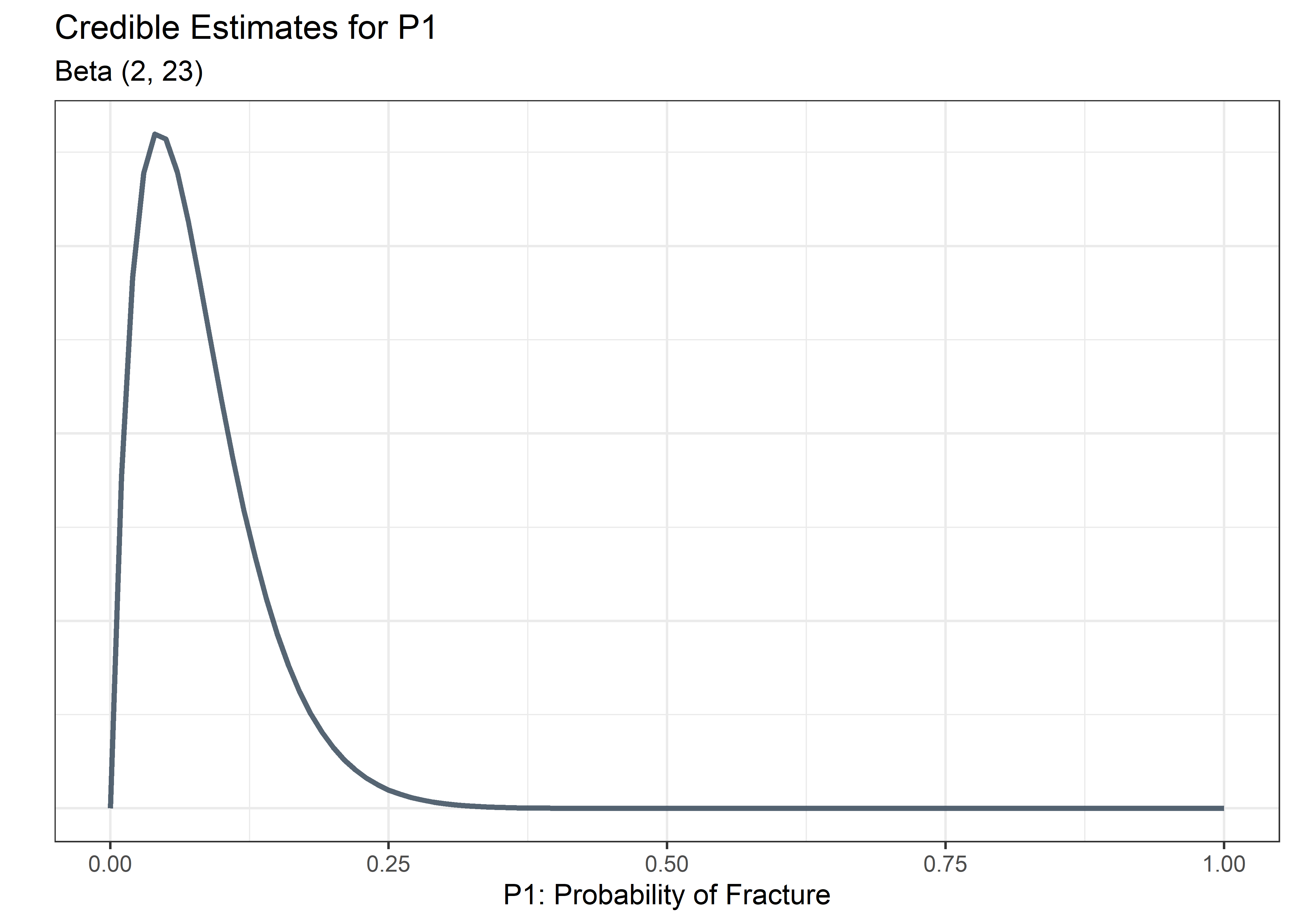
Round 3: 12 parts tested and all 11 passed (1 failure). So we add 11 to the cumulative sum for b and 1 to the cumulative sum for a.
alpha <- 2
beta <- 23

plot_p1_fcn(a = alpha, b = beta)
Pausing here to assess, we can see a wide range of values for P1 that are still consistent with the data, ranging from close to 0 up to around .25.
Model for P2
Now we consider a model for \(\mbox P_2\), the probability of a fracture resulting in a harm (embolism). We can use the same methodology but now we consider additional inputs that are not benchtop data - they are FEA simulations. FEA cannot be thought of as coming from a sampling distribution - if we were to run the FEA simultaion a second time we would get the exact same results (recall that the FEA model suggested no cascading fractures we be expected as a result of the first). Yet this is important knowledge that must inform our risk assessment. So do we give it the impact of a single benchtop data point? No, this would be too little respect for an engineering analysis of this type.
A way that we could incorporate the FEA output is to consider, as subject matter experts, how much weight we intend to place in the FEA simulation. On the one hand we know that FEA can sometimes yield strange predictions due to mesh sensitivities, material model inaccuracies, or assumptions about the boundary conditions. On the other hand, it is a rigorous piece of engineering information coming from validated software that we would be foolish to ignore.
Assume our team of risk modelers meets with the FEA simulation engineers, discusses potential limitations of the FEA, and aligns on a risk estimate centered around .05 but allowing for credible values down to around .2i ish. We could convert this domain knowledge, coming from our FEA, into a prior that reflects this uncertainty. Something like Beta(1,20) should work well.
Combining this knowledge of the FEA along with our benchtop results is how a Bayesian workflow can really shine in ways that our traditional ways can’t.
Prior Probability based on FEA (Input 1)
p_2 <- tibble(x_canvas = c(0, 1))

alpha <- 1
beta <- 20

plot_p2_fcn <- function(a, b) {
  p_2 %>%
    ggplot(aes(x = x_canvas)) +
    stat_function(
      fun = dbeta,
      args = list(a, b),
      color = "firebrick",
      size = 1,
      alpha = .8
    ) +
    #  ylim(c(0, 1.5)) +
    labs(
      y = "",
      x = "P2: Probability of Fracture resulting in Harm",
      title = "Credible Estimates for P2",
      subtitle = str_glue("Beta ({a}, {b})")
    ) +
    theme_bw() +
    theme(
      axis.text.y = element_blank(),
      axis.ticks.y = element_blank()
    )
}

plot_p2_fcn(a = alpha, b = beta) +
  labs(caption = "prior probabilities assessed primarily from FEA")
Add Input 2 (Benchtop Data)
Now we add our study where we looked at 6 parts that were intentionally fractured and saw no propagation or cascading failures. So we add 6 to the cumulative sum for b and nothing to a.
alpha <- 1
beta <- 26

plot_p2_fcn(alpha, beta)
Model for Ph
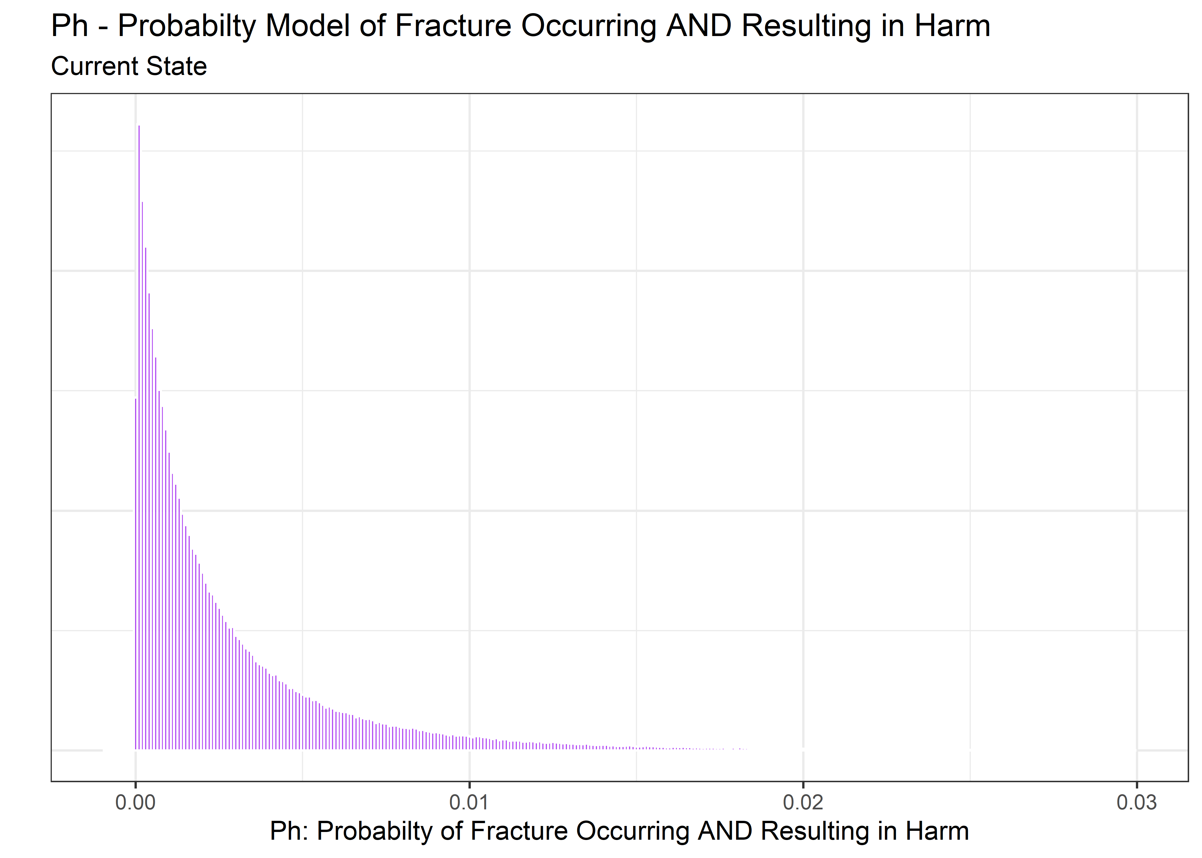
We now have posterior distributions for both \(\mbox P_1\), \(\mbox P_2\), and we need to multiply them together to estimate \(\mbox P_h\). There is probably a way to do this analytically, but most engineers won’t know how beyond multiplying the point estimates. Fortunately we can sample from each of these distributions, multiply the samples together row-wise, and produce an estimate of the posterior for \(\mbox P_h\) that reflects the uncertainty in \(\mbox P_1\) and \(\mbox P_2\).
Sample from P1 Posterior and Visualize
set.seed(123)
n_draws <- 500000

p1_post_draws_tbl <- tibble(draws = rbeta(n = n_draws, shape1 = 2, shape2 = 23))

p1_post_draws_tbl %>%
gt_preview()| draws | |
|---|---|
| 1 | 0.04862055 |
| 2 | 0.06549307 |
| 3 | 0.30463148 |
| 4 | 0.08498940 |
| 5 | 0.08936808 |
| 6..499999 | |
| 500000 | 0.02849358 |
p1_post_draws_tbl %>%
  ggplot(aes(x = draws)) +
  geom_histogram(
    binwidth = .002,
    color = "white",
    fill = "#2c3e50",
    alpha = 0.8
  ) +
  xlim(c(-0.05, .5)) +
  labs(
    y = "",
    title = "Samples from P1 Posterior",
    subtitle = "Current State of Belief",
    x = "P1: Probability of Fracture"
  ) +
  theme_bw() +
  theme(
    axis.text.y = element_blank(),
    axis.ticks.y = element_blank()
  )
Sample from P2 Posterior and Visualize
set.seed(123)
n_draws <- 500000

p2_post_draws_tbl <- tibble(draws = rbeta(n = n_draws, shape1 = 1, shape2 = 26))

p2_post_draws_tbl %>%
gt_preview()| draws | |
|---|---|
| 1 | 0.0526550965 |
| 2 | 0.0024287487 |
| 3 | 0.0332258372 |
| 4 | 0.0303373980 |
| 5 | 0.0017321513 |
| 6..499999 | |
| 500000 | 0.0002236549 |
p2_post_draws_tbl %>%
  ggplot(aes(x = draws)) +
  geom_histogram(
    binwidth = .002,
    color = "white",
    fill = "firebrick",
    alpha = 0.8
  ) +
  xlim(c(-0.05, .5)) +
  labs(
    y = "",
    title = "Samples from P2 Posterior",
    subtitle = "Current State of Belief",
    x = "P2: Probability of a Fracture Resulting in a Harm"
  ) +
  theme_bw() +
  theme(
    axis.text.y = element_blank(),
    axis.ticks.y = element_blank()
  )
Combine to Estimate Ph
joint_post_tbl <- p1_post_draws_tbl %>%
  bind_cols(p2_post_draws_tbl) %>%
  rename(
    p1_draws = draws...1,
    p2_draws = draws...2
  ) %>%
  mutate(p1_x_p2 = p1_draws * p2_draws)

joint_post_tbl %>%
  ggplot(aes(x = p1_x_p2)) +
  geom_histogram(
    binwidth = .0001,
    color = "white",
    fill = "purple",
    alpha = 0.8
  ) +
  labs(
    y = "",
    title = "Ph - Probabilty Model of Fracture Occurring AND Resulting in Harm",
    subtitle = "Current State",
    x = "Ph: Probabilty of Fracture Occurring AND Resulting in Harm"
  ) +
  theme_bw() +
  theme(
    axis.text.y = element_blank(),
    axis.ticks.y = element_blank()
  ) +
  xlim(c(-.001, .03))
The above plot can also be summarized in tabular form.
joint_post_tbl %>%
  select(p1_x_p2) %>%
  mutate_if(is.numeric, round, 4) %>%
  median_qi(.width = .95) %>%
  gt() %>%
  cols_align("center") %>%
  opt_row_striping(row_striping = TRUE) %>%
  tab_header(
    title = "Summary of Ph Posterior",
    subtitle = "Based on Bayesian Beta/Binomial Model"
  ) %>%
  cols_width(everything() ~ px(100)) %>%
  tab_style(
    style = list(
      cell_text(weight = "bold")
    ),
    locations = cells_column_labels(columns = everything())
)| Summary of Ph Posterior | |||||
|---|---|---|---|---|---|
| Based on Bayesian Beta/Binomial Model | |||||
| p1_x_p2 | .lower | .upper | .width | .point | .interval |
| 0.0016 | 0 | 0.014 | 0.95 | median | qi |
We have arrived at an estimate for Ph, the probability of the fracture occurring and resulting in a harm. A point estimate is .0016 or 16 out of 1000. A decision made off this single value may result in pushing a product that seems relatively safe. But the 95% credible interval covers up to .014 or 1.4 in 100 which would not be acceptable in most circumstances. The Bayesian approach has allowed us to carry that uncertainty all the way through the calculations to make a more informed decision.
This is the distillation of a lot of work to prepare the problem for a business decision: do nothing, initiate a redesign, or proceed with more testing.
In this hypothetical example, credible risk values above 1% are likely too high to proceed without design changes or additional testing.
If you’ve made it this far, I thank you for your attention.
SessionInfo
sessionInfo()## R version 4.0.3 (2020-10-10)
## Platform: x86_64-w64-mingw32/x64 (64-bit)
## Running under: Windows 10 x64 (build 18363)
##
## Matrix products: default
##
## locale:
## [1] LC_COLLATE=English_United States.1252
## [2] LC_CTYPE=English_United States.1252
## [3] LC_MONETARY=English_United States.1252
## [4] LC_NUMERIC=C
## [5] LC_TIME=English_United States.1252
##
## attached base packages:
## [1] stats graphics grDevices utils datasets methods base
##
## other attached packages:
## [1] tidybayes_2.3.1 gt_0.2.2 forcats_0.5.0 stringr_1.4.0
## [5] dplyr_1.0.7 purrr_0.3.4 readr_1.4.0 tidyr_1.1.3
## [9] tibble_3.1.4 ggplot2_3.3.5 tidyverse_1.3.0
##
## loaded via a namespace (and not attached):
## [1] Rcpp_1.0.7 lattice_0.20-41 lubridate_1.7.9.2
## [4] assertthat_0.2.1 digest_0.6.28 utf8_1.2.2
## [7] plyr_1.8.6 R6_2.5.1 cellranger_1.1.0
## [10] backports_1.2.0 reprex_0.3.0 evaluate_0.14
## [13] coda_0.19-4 highr_0.9 httr_1.4.2
## [16] blogdown_0.15 pillar_1.6.2 rlang_0.4.11
## [19] readxl_1.3.1 rstudioapi_0.13 jquerylib_0.1.4
## [22] checkmate_2.0.0 rmarkdown_2.11 labeling_0.4.2
## [25] munsell_0.5.0 broom_0.7.8 compiler_4.0.3
## [28] modelr_0.1.8 xfun_0.26 pkgconfig_2.0.3
## [31] htmltools_0.5.2 tidyselect_1.1.1 bookdown_0.21
## [34] arrayhelpers_1.1-0 fansi_0.5.0 crayon_1.4.1
## [37] dbplyr_2.0.0 withr_2.4.2 distributional_0.2.1
## [40] ggdist_2.3.0 grid_4.0.3 jsonlite_1.7.2
## [43] gtable_0.3.0 lifecycle_1.0.1 DBI_1.1.0
## [46] magrittr_2.0.1 scales_1.1.1 cli_3.0.1
## [49] stringi_1.7.4 farver_2.1.0 fs_1.5.0
## [52] xml2_1.3.2 bslib_0.3.0 ellipsis_0.3.2
## [55] generics_0.1.0 vctrs_0.3.8 tools_4.0.3
## [58] svUnit_1.0.3 glue_1.4.2 hms_0.5.3
## [61] fastmap_1.1.0 yaml_2.2.1 colorspace_2.0-2
## [64] rvest_0.3.6 knitr_1.34 haven_2.3.1
## [67] sass_0.4.0https://www.greenlight.guru/blog/en-iso-149712012-risk-assessment-explained↩︎
We will ignore the Severity adjustment typically involved in risk calculations per EN ISO 14971 for simplicity↩︎
https://nitinol.com/wp-content/uploads/2017/11/a666400cdba78b589ce578e17fc2c3fd.pdf↩︎