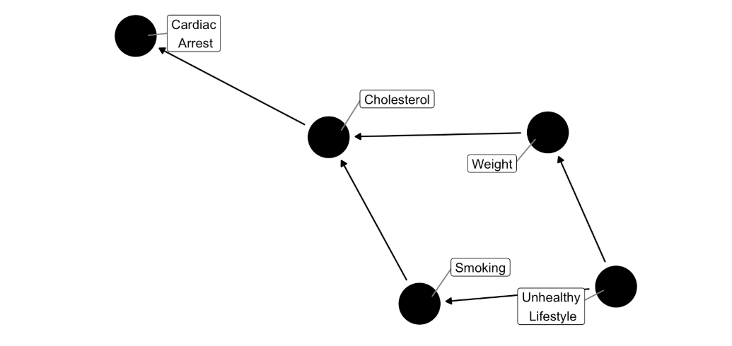
Like many engineers, my first models were based on Designed Experiments in the tradition of Cox and Montgomery. I hadn’t seen anything like a causal diagram until I picked the The Book of Why which explores all sorts of experimental relationships and structures I never imagined.1 Colliders, confounders, causal diagrams, M-bias - these concepts are all relatively new to me and I want to understand them better. In this post I will attempt to create some simple structural causal models (SCMs) for myself using the Dagitty and GGDag packages and then show the potential effects of confounders and colliders on a simulated experiment adapted from here.2
It turns out that it is not as simple as identifying lurking variables and holding them constant while we conduct the experiment of interest (as I was always taught).
First, load the libraries.
# Load libraries
library(tidyverse)
library(kableExtra)
library(tidymodels)
library(viridisLite)
library(GGally)
library(dagitty)
library(ggdag)
library(visreg)
library(styler)
library(cowplot)
A structural causal model (SCM) is a type of directed acyclic graph (DAG) that maps causal assumptions onto a simple model of experimental variables. In the figure below, each node(blue dot) represents a variable. The edges(yellow lines) between nodes represent assumed causal effects.
Dagitty uses the dafigy() function to create the relationships in the DAG. These are stored in a DAG object which is provided to ggplot and can then be customized and adjusted. Most of the code below the DAG object is just formatting the figure.
# create DAG object
g <- dagify(
A ~ J,
X ~ J,
X ~ A
)
# tidy the dag object and supply to ggplot
set.seed(100)
g %>%
tidy_dagitty() %>%
mutate(x = c(0, 1, 1, 2)) %>%
mutate(y = c(0, 2, 2, 0)) %>%
mutate(xend = c(2, 0, 2, NA)) %>%
mutate(yend = c(0, 0, 0, NA)) %>%
dag_label(labels = c(
"A" = "Independent\n Variable",
"X" = "Dependent\n Variable",
"J" = "The\n Confounder"
)) %>%
ggplot(aes(x = x, y = y, xend = xend, yend = yend)) +
geom_dag_edges(
edge_colour = "#b8de29ff",
edge_width = .8
) +
geom_dag_node(
color = "#2c3e50",
alpha = 0.8
) +
geom_dag_text(color = "white") +
geom_dag_label_repel(aes(label = label),
col = "white",
label.size = .4,
fill = "#20a486ff",
alpha = 0.8,
show.legend = FALSE,
nudge_x = .7,
nudge_y = .3
) +
labs(
title = " Directed Acyclic Graph",
subtitle = " Two Variables of Interest with a Confounder"
) +
xlim(c(-1.5, 3.5)) +
ylim(c(-.33, 2.2)) +
geom_rect(
xmin = -.5,
xmax = 3.25,
ymin = -.25,
ymax = .65,
alpha = .04,
fill = "white"
) +
theme_void() +
theme(
plot.background = element_rect(fill = "#222222"),
plot.title = element_text(color = "white"),
plot.subtitle = element_text(color = "white")
)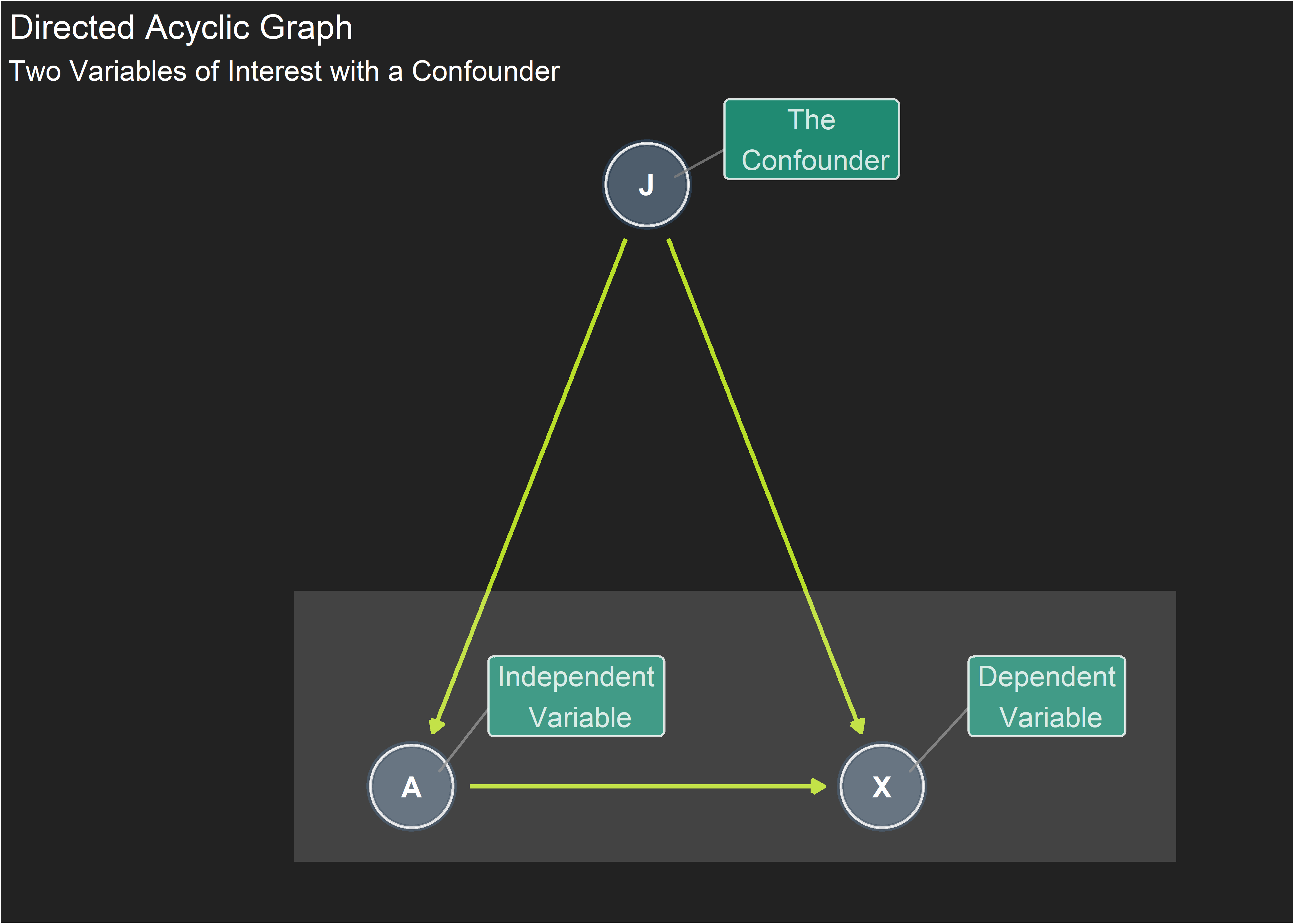 The relationship of interest is captured in the lower rectangle: we want to change the value of independent variable A and record the effect on dependent variable X (in epidemiology these might be called “treatment” and “outcome”). There also happens to be a confounding variable J that has a causal effect on both A and X.
We can set up a simulated experiment that follows the structure of the SCM above:
Each variable will have n=1000 values. J is generated by drawing randomly from a standard normal distribution. We want J to be a cause of A so we use J in the creation of A along with a random error term to represent noise. The model above shows a causal link from A to X but we don’t actually know if this exists - that’s the point of the experiment. It may or may not be there (from the point of view of the experimenter/engineer). For the purposes of demonstration we will structure the simulation such that there is no causal relationship between A and X (A will not be used in the creation of the variable J). Again we need J as a cause of X so we use J in the creation of the dependent_var_X object along with a random noise component.
The simulation is now set up to model an experiment where the experimenter/engineer wants to understand the effect of A on X but the true effect is zero. Meanwhile, there is a confounding variable J that is a parent to both A and X.
# set seed for repeatability
set.seed(805)

# n = 1000 points for the simulation
n <- 1000

# create variables
# J is random draws from standard normal (mean = 0, stdev = 1)
confounding_var_J <- rnorm(n)

# J is used in creation of A since it is a cause of A (confounder)
independent_var_A <- 1.1 * confounding_var_J + rnorm(n)

# J is used in creation of X since it is a cause of X (confounder)
dependent_var_X <- 1.9 * confounding_var_J + rnorm(n)
In reality, the experimenter may or may not be aware of the parent confounder J. We will create two different regression models below. In the first, denoted crude_model, we will assume the experimenter was unaware of the confounder. The model is then created with A as the only predictor variable of X.
In the second, denoted confounder_model, we will assume the experimenter was aware of the confounder and chose to include it in their model. This version is created with A and J as predictors of X.
# create crude regression model with A predicting X.  J is omitted
crude_model <- lm(dependent_var_X ~ independent_var_A)

# create confounder model with A and J predicting X
confounder_model <- lm(dependent_var_X ~ independent_var_A + confounding_var_J)

# tidy the crude model and examine it
crude_model_tbl <- summary(crude_model) %>% tidy()
crude_model_kbl <- summary(crude_model) %>%
  tidy() %>%
  kable(align = rep("c", 5), digits = 3)
crude_model_kbl| term | estimate | std.error | statistic | p.value |
|---|---|---|---|---|
| (Intercept) | -0.007 | 0.051 | -0.135 | 0.893 |
| independent_var_A | 0.967 | 0.034 | 28.415 | 0.000 |
# Tidy the confounder model and examine it
confounder_model_tbl <- summary(confounder_model) %>% tidy()
confounder_model_kbl <- summary(confounder_model) %>%
  tidy() %>%
  kable(align = rep("c", 5), digits = 3)
confounder_model_kbl| term | estimate | std.error | statistic | p.value |
|---|---|---|---|---|
| (Intercept) | -0.005 | 0.032 | -0.151 | 0.880 |
| independent_var_A | 0.005 | 0.033 | 0.153 | 0.878 |
| confounding_var_J | 1.860 | 0.048 | 38.460 | 0.000 |
# add column for labels
crude_model_tbl <- crude_model_tbl %>% mutate(model = "crude_model: no confounder")
confounder_model_tbl <- confounder_model_tbl %>% mutate(model = "confounder_model: with confounder")

# combine into a single kable
confounder_model_summary_tbl <- bind_rows(crude_model_tbl, confounder_model_tbl)
confounder_model_summary_tbl <- confounder_model_summary_tbl %>% select(model, everything())
confounder_model_summary_tbl %>% kable(align = rep("c", 6), digits = 3)| model | term | estimate | std.error | statistic | p.value |
|---|---|---|---|---|---|
| crude_model: no confounder | (Intercept) | -0.007 | 0.051 | -0.135 | 0.893 |
| crude_model: no confounder | independent_var_A | 0.967 | 0.034 | 28.415 | 0.000 |
| confounder_model: with confounder | (Intercept) | -0.005 | 0.032 | -0.151 | 0.880 |
| confounder_model: with confounder | independent_var_A | 0.005 | 0.033 | 0.153 | 0.878 |
| confounder_model: with confounder | confounding_var_J | 1.860 | 0.048 | 38.460 | 0.000 |
The combined summary table above provides the effect sizes and the difference between the two models is striking. Conditional plots are a way to visualize regression models. The visreg package creates conditional plots by supplying a model object and a predictor variable to the visreg() function. The x-axis shows the value of the predictor variable and the y-axis shows change in the response variable. All other variables are held constant at their medians.
# visualize conditional plot of A vs X, crude model
v1 <- visreg(crude_model,
  "independent_var_A",
  gg = TRUE,
  line = list(col = "#E66101")
) +
  labs(
    title = "Relationship Between A and X",
    subtitle = "Neglecting Confounder Variable J"
  ) +
  ylab("Change in Response X") +
  ylim(-6, 6) +
  theme(plot.subtitle = element_text(face = "bold", color = "#404788FF"))

# visualize conditional plot of A vs X, confounder model
v2 <- visreg(confounder_model,
  "independent_var_A",
  gg = TRUE,
  line = list(col = "#E66101")
) +
  labs(
    title = "Relationship Between A and X",
    subtitle = "Considering Confounder Variable J"
  ) +
  ylab("Change in Response X") +
  ylim(-6, 6) +
  theme(plot.subtitle = element_text(face = "bold", color = "#20a486ff"))

plot_grid(v1, v2)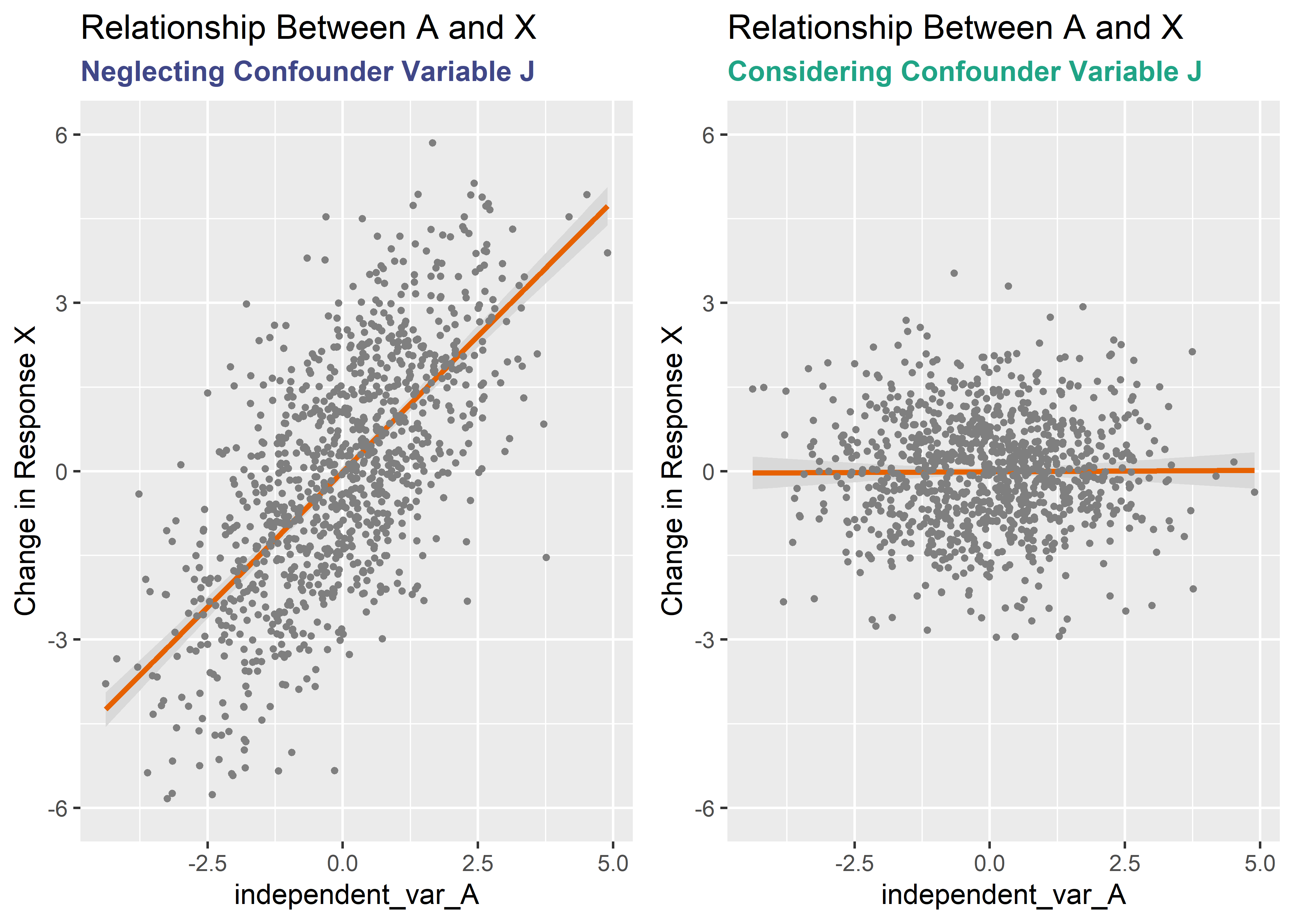
We know from creating the simulated data that A has no real effect on the outcome X. X was created using only J and some noise. But the left plot shows a large, positive slope and significant coefficient! How can this be? This faulty estimate of the true effect is biased; more specifically we are seeing “confounder bias” or “omitted variable bias”. Adding J to the regression model has the effect of conditioning on J and revealing the true relationship between A and X: no effect of A on X.
Confounding is pretty easy to understand. “Correlation does not imply causation” has been drilled into my brain effectively. Still, confounders that aren’t anticipated can derail studies and confuse observers. For example, the first generation of drug eluting stents was released in the early 2000’s. They showed great promise but their long-term risk profile was not well understood. Observational studies indicated an improved mortality rate for drug-eluting stents relative to their bare-metal counterparts. However, the performance benefit could not be replicated in randomized controlled trials.3
The disconnect was eventually linked (at least in part) to a confounding factor. Outside of a RCT, clinicians took into account the health of the patient going into the procedure. Specifically, if the patient was scheduled for a pending surgery or had a history of clotting then the clinician would hedge towards a bare-metal stent (since early gen DES tended to have thrombotic events at a greater frequency than BMS). Over the long term, these sicker patients were assigned BMS disproportionately, biasing the effect of stent type on long-term mortality via patient health as a confounder.
So we always want to include every variable we know about in our regression models, right? Wrong. Here is a case that looks similar to the confounder scenario but is slightly different. The question of interest is the same: evaluate the effect of predictor B on the outcome Y. Again, there is a 3rd variable at play. But this time, the third variable is caused by both B and Y rather than being itself the common cause.
# assign DAG object
h <- dagify(
  K ~ B + Y,
  Y ~ B
)

# tidy the dag object and suppply to ggplot
set.seed(100)
h %>%
  tidy_dagitty() %>%
  mutate(x = c(0, 0, 2, 1)) %>%
  mutate(y = c(0, 0, 0, 2)) %>%
  mutate(xend = c(1, 2, 1, NA)) %>%
  mutate(yend = c(2, 0, 2, NA)) %>%
  dag_label(labels = c(
    "B" = "Independent\n Variable",
    "Y" = "Dependent\n Variable",
    "K" = "The\n Collider"
  )) %>%
  ggplot(aes(x = x, y = y, xend = xend, yend = yend)) +
  geom_dag_edges(
    edge_colour = "#b8de29ff",
    edge_width = .8
  ) +
  geom_dag_node(
    color = "#2c3e50",
    alpha = 0.8
  ) +
  geom_dag_text(color = "white") +
  geom_dag_label_repel(aes(label = label),
    col = "white",
    label.size = .4,
    fill = "#20a486ff",
    alpha = 0.8,
    show.legend = FALSE,
    nudge_x = .7,
    nudge_y = .3
  ) +
  labs(
    title = " Directed Acyclic Graph",
    subtitle = " Two Variables of Interest with a Collider"
  ) +
  xlim(c(-1.5, 3.5)) +
  ylim(c(-.33, 2.2)) +
  geom_rect(
    xmin = -.5,
    xmax = 3.25,
    ymin = -.25,
    ymax = .65,
    alpha = .04,
    fill = "white"
  ) +
  theme_void() +
  theme(
    plot.background = element_rect(fill = "#222222"),
    plot.title = element_text(color = "white"),
    plot.subtitle = element_text(color = "white")
  )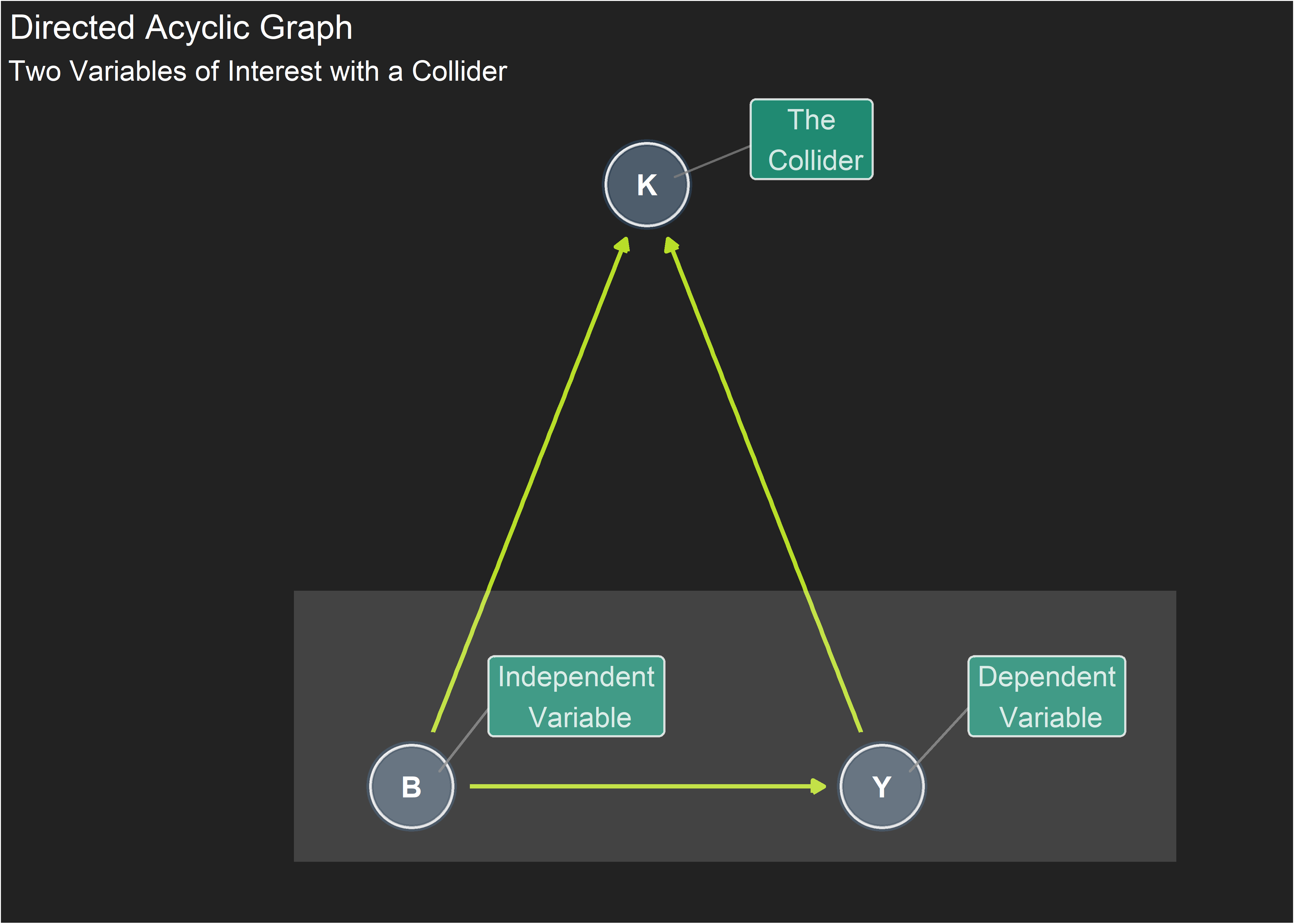
A variable like this is called a collider because the causal arrows from from B and Y collide at K. K is created in the simulation below using both B and Y plus random noise. This time, the outcome Y is created using B as an input, thereby assigning a causal relation with an effect size of 0.3.
# create variables
# B is random draws from standard normal (mean = 0, stdev = 1)
independent_var_B <- rnorm(n)

# Y is created with B and noise. Effect size of B on Y is 0.3
dependent_var_Y <- .3 * independent_var_B + rnorm(n)

# K (collider) is created with B and Y + noise
collider_var_K <- 1.2 * independent_var_B + 0.9 * dependent_var_Y + rnorm(n)
Let’s assume that the experimenter knows about possible collider variable K. What should they do with it when they go to create their regression model? Let’s create two models again to compare results. Following the nomenclature from before: crude_model_b uses only B to predict Y and collider_model uses both B and K to predict Y.
# create crude regression model with B predicting Y.  K is omitted
crude_model_b <- lm(dependent_var_Y ~ independent_var_B)

# create collider model with B and K predicting Y
collider_model <- lm(dependent_var_Y ~ independent_var_B + collider_var_K)

# tidy the crude model and examine it
crude_model_b_kbl <- summary(crude_model_b) %>%
  tidy() %>%
  kable(align = rep("c", 5), digits = 3)
crude_model_b_tbl <- summary(crude_model_b) %>% tidy()
crude_model_b_kbl| term | estimate | std.error | statistic | p.value |
|---|---|---|---|---|
| (Intercept) | -0.021 | 0.032 | -0.666 | 0.506 |
| independent_var_B | 0.247 | 0.032 | 7.820 | 0.000 |
# tidy the collider model and examine it
collider_model_kbl <- summary(collider_model) %>%
  tidy() %>%
  kable(align = rep("c", 5), digits = 3)
collider_model_tbl <- summary(collider_model) %>% tidy()
collider_model_kbl| term | estimate | std.error | statistic | p.value |
|---|---|---|---|---|
| (Intercept) | -0.011 | 0.023 | -0.453 | 0.651 |
| independent_var_B | -0.481 | 0.034 | -14.250 | 0.000 |
| collider_var_K | 0.519 | 0.018 | 29.510 | 0.000 |
# add label column
crude_model_b_tbl <- crude_model_b_tbl %>% mutate(model = "crude_model_b: no collider")
collider_model_tbl <- collider_model_tbl %>% mutate(model = "collider_model: with collider")

# combine and examine
collider_model_summary_tbl <- bind_rows(crude_model_b_tbl, collider_model_tbl)
collider_model_summary_tbl <- collider_model_summary_tbl %>% select(model, everything())
collider_model_summary_tbl %>% kable(align = rep("c", 6), digits = 3)| model | term | estimate | std.error | statistic | p.value |
|---|---|---|---|---|---|
| crude_model_b: no collider | (Intercept) | -0.021 | 0.032 | -0.666 | 0.506 |
| crude_model_b: no collider | independent_var_B | 0.247 | 0.032 | 7.820 | 0.000 |
| collider_model: with collider | (Intercept) | -0.011 | 0.023 | -0.453 | 0.651 |
| collider_model: with collider | independent_var_B | -0.481 | 0.034 | -14.250 | 0.000 |
| collider_model: with collider | collider_var_K | 0.519 | 0.018 | 29.510 | 0.000 |
This time, omitting the collider variable is the proper way to recover the true effect of B on Y. Let’s verify with conditional plots as before. Again, we know the true slope should be around 0.3.
# create conditional plot with crude_model_b and B
v3 <- visreg(crude_model_b,
"independent_var_B",
gg = TRUE,
line = list(col = "#E66101")
) +
labs(
title = "Relationship Between B and Y",
subtitle = "Neglecting Collider Variable K"
) +
ylab("Change in Response Y") +
ylim(-6, 6) +
theme(plot.subtitle = element_text(face = "bold", color = "#f68f46b2"))
# create conditional plot with collider_model and B
v4 <- visreg(collider_model,
"independent_var_B",
gg = TRUE,
line = list(col = "#E66101")
) +
labs(
title = "Relationship Between B and Y",
subtitle = "Considering Collider Variable K"
) +
ylab("Change in Response Y") +
ylim(-6, 6) +
theme(plot.subtitle = element_text(face = "bold", color = "#403891b2"))
plot_grid(v3, v4)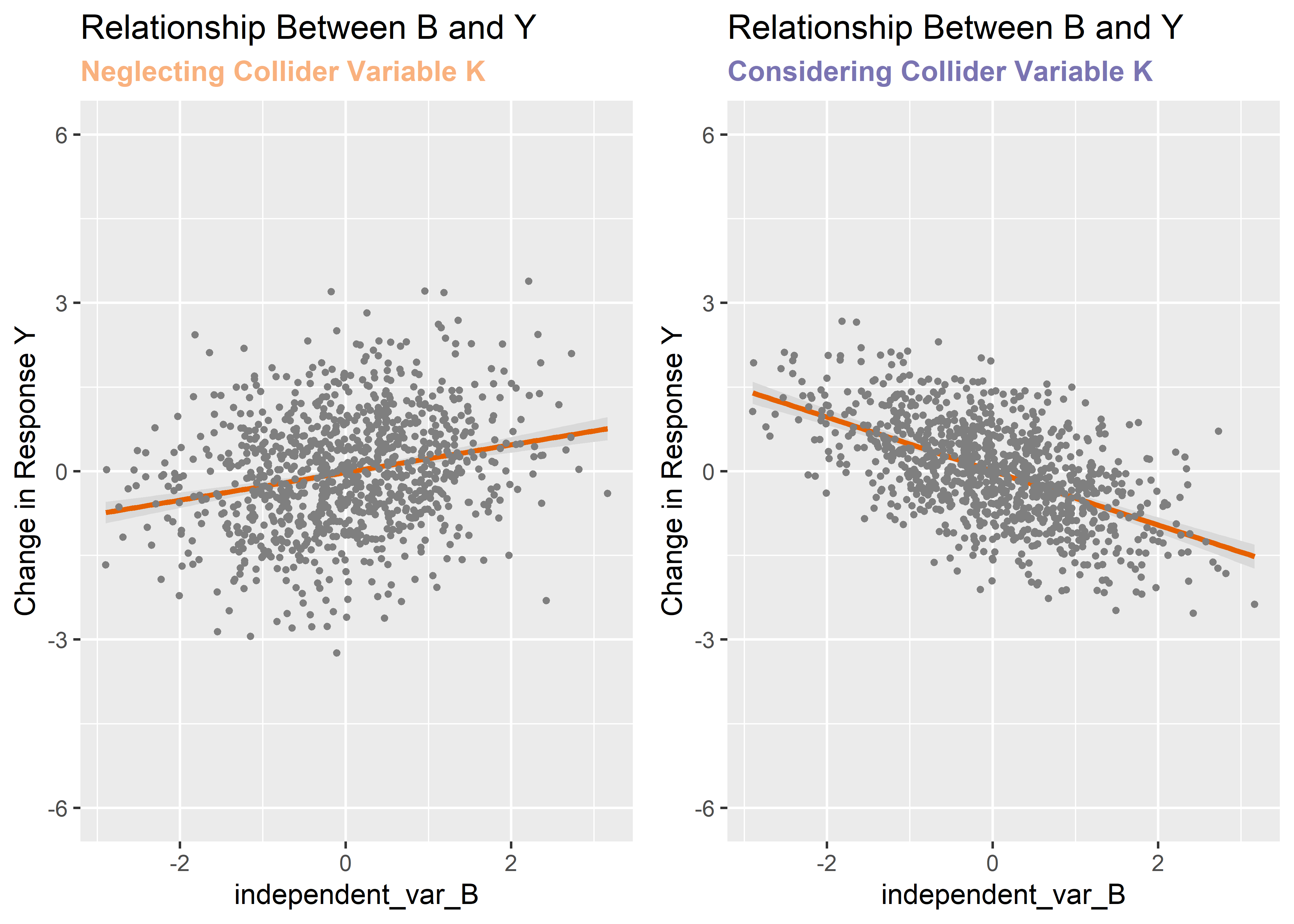 Incredibly, the conclusion one draws about the relationship between B and Y completely reverses depending upon which model is used. The true effect is positive (we only know this for sure because we created the data) but by including the collider variable in the model we observe it as negative. We should not control for a collider variable!
Controlling for a confounder reduces bias but controlling for a collider increases it - a simple summary that I will try to remember as I design future experiments or attempt to derive meaning from observational studies. These are the simple insights that make learning this stuff really fun (for me at least)!
Thanks for reading.