Tolerance intervals are used to specify coverage of a population of data. In the frequentist framework, the width of the interval is dependent on the desired coverage proportion and the specified confidence level. They are widely used in the medical device industry because they can be compared directly vs. product specifications, allowing the engineer to make a judgment about what percentage of the parts would meet the spec taking into account sampling uncertainty.
In this post I wanted to dive a bit deeper into the frequentist version of tolerance intervals to verify that they provide the correct coverage in a straight-forward use case. Then I will explore a Bayesian version which uses the posterior draws from a fitted model to calculate the Bayesian analogue of a tolerance interval.
Libraries
library(tidyverse)
library(here)
library(brms)
library(broom)
library(tidybayes)
library(tolerance)
library(wesanderson)
library(patchwork)
library(gt)
As with any frequentist simulation looking at coverage of a p-value, we can start with the population parameters known. From there we simulate many draws from that population and calculate the desired statistic (in this case the tolerance interval limits). By comparing each calculated tolerance interval to the true population coverage, we can determine the number of simulations that do not meet the specified coverage. If that number, as a fraction of the total number of sims, is less than or equal to the p-value, then the tolerance interval procedure is working as intended and provided the specified coverage, on average, over many simulated experiments.
This block sets up the parameters and identifies the specified quantiles of the true population.
Simulated Experiments
True Population Parameters
set.seed(9989)

n_sims <- 10000
true_population_mean <- 40
true_population_sd <- 4
alpha <- 0.1
p <- .95

upper_97.5 <- qnorm(p = .975, mean = true_population_mean, sd = true_population_sd)
lower_02.5 <- qnorm(p = .025, mean = true_population_mean, sd = true_population_sd)
Now run the simulation, replicating many “experiments” of n=15, calculating a 90% confidence, 2-sided tolerance interval for 95% of the population each time.
Run the Simulation
sim_summary_tbl <- tibble(sim_id = seq(from = 1, to = n_sims, by = 1)) %>%
  rowwise() %>%
  mutate(
    test_sample_size = 15,
    sim_test_data = list(rnorm(n = test_sample_size, mean = true_population_mean, sd = true_population_sd))
  ) %>%
  summarize(
    sim_id = sim_id,
    #   sim_test_data = sim_test_data,
    norm_tol = list(normtol.int(sim_test_data, alpha = alpha, P = p, side = 2)),
    sample_sd = sd(sim_test_data)
  ) %>%
  unnest(norm_tol) %>%
  rename(
    lower_bound_ltl = "2-sided.lower",
    upper_bound_utl = "2-sided.upper",
    sample_mean = x.bar,
    p = P
  ) %>%
  ungroup() %>%
  select(sim_id, alpha, p, sample_mean, sample_sd, everything()) %>%
  mutate(
    true_lower_2.5 = lower_02.5,
    true_upper_97.5 = upper_97.5
  )

sim_summary_tbl %>%
gt_preview()| sim_id | alpha | p | sample_mean | sample_sd | lower_bound_ltl | upper_bound_utl | true_lower_2.5 | true_upper_97.5 | |
|---|---|---|---|---|---|---|---|---|---|
| 1 | 1 | 0.1 | 0.95 | 36.19320 | 3.243531 | 27.35493 | 45.03147 | 32.16014 | 47.83986 |
| 2 | 2 | 0.1 | 0.95 | 40.56155 | 3.766514 | 30.29821 | 50.82489 | 32.16014 | 47.83986 |
| 3 | 3 | 0.1 | 0.95 | 40.23154 | 4.268292 | 28.60091 | 51.86217 | 32.16014 | 47.83986 |
| 4 | 4 | 0.1 | 0.95 | 40.24057 | 4.175918 | 28.86165 | 51.61949 | 32.16014 | 47.83986 |
| 5 | 5 | 0.1 | 0.95 | 40.41020 | 3.880094 | 29.83737 | 50.98303 | 32.16014 | 47.83986 |
| 6..9999 | |||||||||
| 10000 | 10000 | 0.1 | 0.95 | 38.69646 | 4.780010 | 25.67145 | 51.72147 | 32.16014 | 47.83986 |
Visualize
Plot the resulting upper and lower bounds of the 90/95 tolerance interval. The red lines are the true population quantiles.
sim_summary_tbl %>%
  pivot_longer(cols = everything(), names_to = "param", values_to = "value") %>%
  filter(param == "lower_bound_ltl" | param == "upper_bound_utl") %>%
  mutate(param = as_factor(param)) %>%
  ggplot(aes(x = value, y = param)) +
  geom_jitter(aes(color = param), width = .1, height = .1, size = .3, alpha = .05) +
  stat_halfeye(aes(fill = param), alpha = .7, position = position_nudge(y = .2)) +
  geom_vline(xintercept = mean(sim_summary_tbl$true_lower_2.5), color = "firebrick", linetype = 2) +
  geom_vline(xintercept = mean(sim_summary_tbl$true_upper_97.5), color = "firebrick", linetype = 2) +
  scale_color_manual(values = wes_palette("Moonrise2")) +
  scale_fill_manual(values = wes_palette("Moonrise2")) +
  #  scale_color_manual(values = c("purple", "limegreen")) +
  #  scale_fill_manual(values = c("purple", "limegreen")) +
  labs(
    x = "",
    y = "",
    title = "Distribution of Calculated Upper and Lower Tolerance Limits",
    subtitle = "10,000 Simulations of n=15 parts with 2-sided normal Tolerance Intervals",
    caption = "pink vertical lines represent true population quantiles, .025 and .975"
  ) +
  theme(
    legend.title = element_blank(),
    legend.position = "bottom"
  )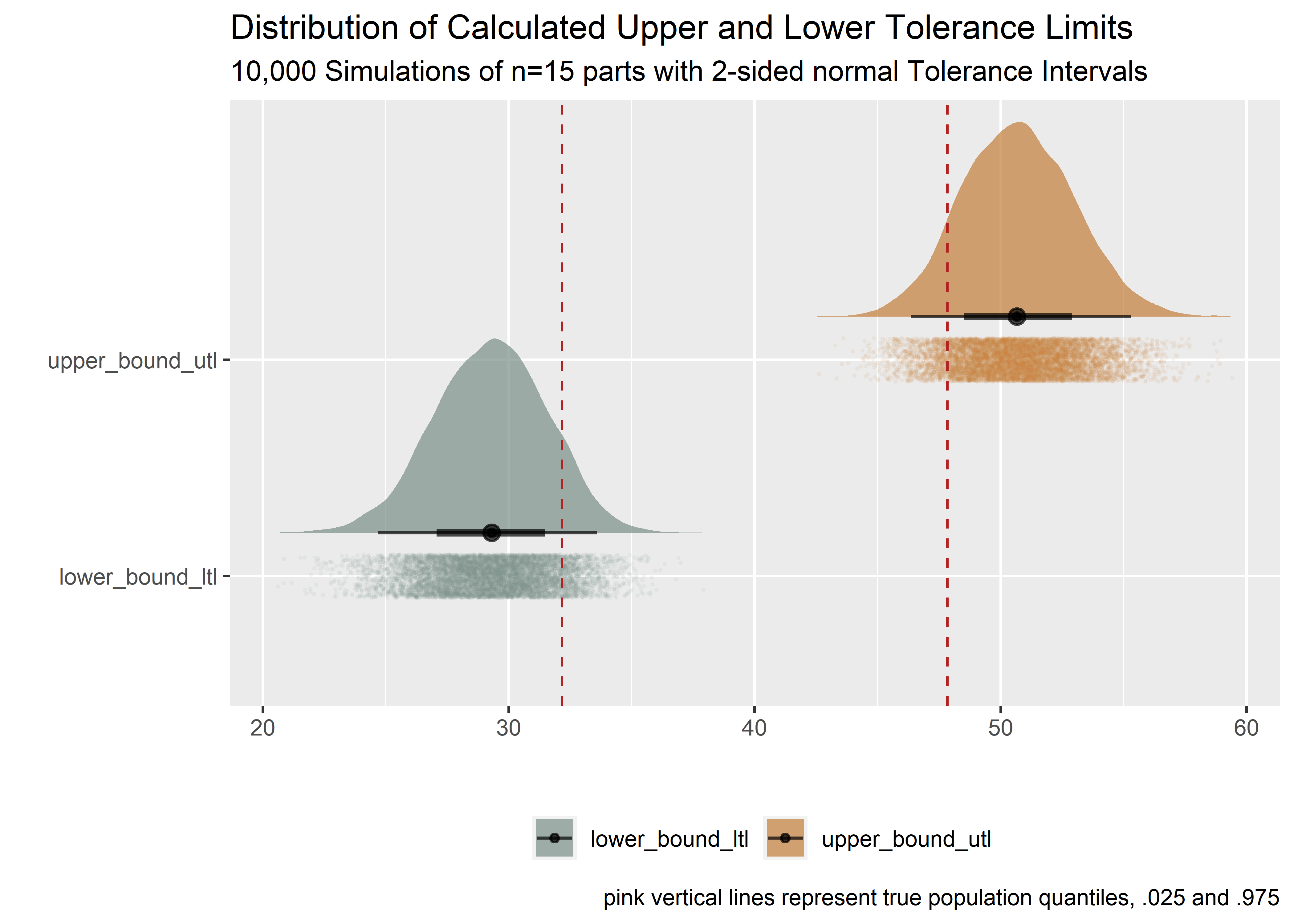
To see if the tolerance interval procedure is providing the desired coverage, we have to look at each set of lower and upper limits from each simulation. The code below converts the calculated tolerance bounds from each sim into quantiles of the true population, then calculates the difference to determine the true population coverage of the simulated experiment. If the coverage is less than intended, a flag of 1 is assigned in the “unacceptable_coverage” col, else 0.
Evaluate True Coverage of Each Simulated Experiment
coverage_summary_tbl <- sim_summary_tbl %>%
  mutate(
    ltl_coverage_true = map_dbl(lower_bound_ltl, pnorm, true_population_mean, true_population_sd),
    utl_coverage_true = map_dbl(upper_bound_utl, pnorm, true_population_mean, true_population_sd)
  ) %>%
  mutate(total_tl_coverage_true = utl_coverage_true - ltl_coverage_true) %>%
  mutate(unacceptable_coverage = case_when(
    total_tl_coverage_true >= p ~ 0,
    TRUE ~ 1
  )) %>%
  select(-c(alpha, p, true_lower_2.5, true_upper_97.5))

coverage_summary_tbl %>%
gt_preview()| sim_id | sample_mean | sample_sd | lower_bound_ltl | upper_bound_utl | ltl_coverage_true | utl_coverage_true | total_tl_coverage_true | unacceptable_coverage | |
|---|---|---|---|---|---|---|---|---|---|
| 1 | 1 | 36.19320 | 3.243531 | 27.35493 | 45.03147 | 0.0007854236 | 0.8957802 | 0.8949948 | 1 |
| 2 | 2 | 40.56155 | 3.766514 | 30.29821 | 50.82489 | 0.0076447723 | 0.9965973 | 0.9889526 | 0 |
| 3 | 3 | 40.23154 | 4.268292 | 28.60091 | 51.86217 | 0.0021875221 | 0.9984893 | 0.9963017 | 0 |
| 4 | 4 | 40.24057 | 4.175918 | 28.86165 | 51.61949 | 0.0026797862 | 0.9981630 | 0.9954832 | 0 |
| 5 | 5 | 40.41020 | 3.880094 | 29.83737 | 50.98303 | 0.0055321969 | 0.9969814 | 0.9914492 | 0 |
| 6..9999 | |||||||||
| 10000 | 10000 | 38.69646 | 4.780010 | 25.67145 | 51.72147 | 0.0001703976 | 0.9983072 | 0.9981368 | 0 |
Count False Positives
For the coverage to be correct, the percentage of false positives (simulated experiments that covered less than p% of the true population) should be less than or equal to alpha (10%). That would mean less than .1(10000) = 1000 cases where the tolerance interval covered less than 95% of the true population.
coverage_summary_tbl %>%
  summarize(
    false_positives = sum(unacceptable_coverage),
    false_positive_limit = alpha * n_sims
  ) %>%
  mutate(
    alpha_level = alpha,
    total_trials = n_sims,
    false_positive_rate = false_positives / n_sims,
    "tol_limit_procedure_working?" = case_when(
      false_positives < false_positive_limit ~ "heck_yes",
      TRUE ~ "boo"
    )
  ) %>%
  select(total_trials, alpha_level, false_positive_limit, everything()) %>%
gt_preview()| total_trials | alpha_level | false_positive_limit | false_positives | false_positive_rate | tol_limit_procedure_working? | |
|---|---|---|---|---|---|---|
| 1 | 10000 | 0.1 | 1000 | 958 | 0.0958 | heck_yes |
Because .0958 is less than .1 (10%) we can say that the tolerance interval procedure is capturing the desired population proportion (95%) with an acceptable false positive rate (<= 10%). Neat!
Bayesian 2-sided Tolerance Interval
Now let’s look at the Bayesian approach. Note that this is completely different example from above, not a continuation. The desired coverage for this case is a little bit different - 95%, and we’ll aim for a 90% confidence level (for the frequentist version that comes later) and we’ll try to capture the 90% most credible estimates for the Bayesian version.
Load the Data
The dataset and example used for this section is adapted from this excellent paper on coverage intervals.1 The values represent measurements of mass fraction of iron made by the National Institute of Standards and Technology (NIST). Units of measurement are percentages, or cg/g.
w_tbl <- tibble(w = c(
67.43, 66.97, 67.65, 66.84, 67.05, 66.57, 67.16, 68.3,
67.01, 67.07, 67.23, 66.51, 66.46, 67.54, 67.09, 66.77
)) %>%
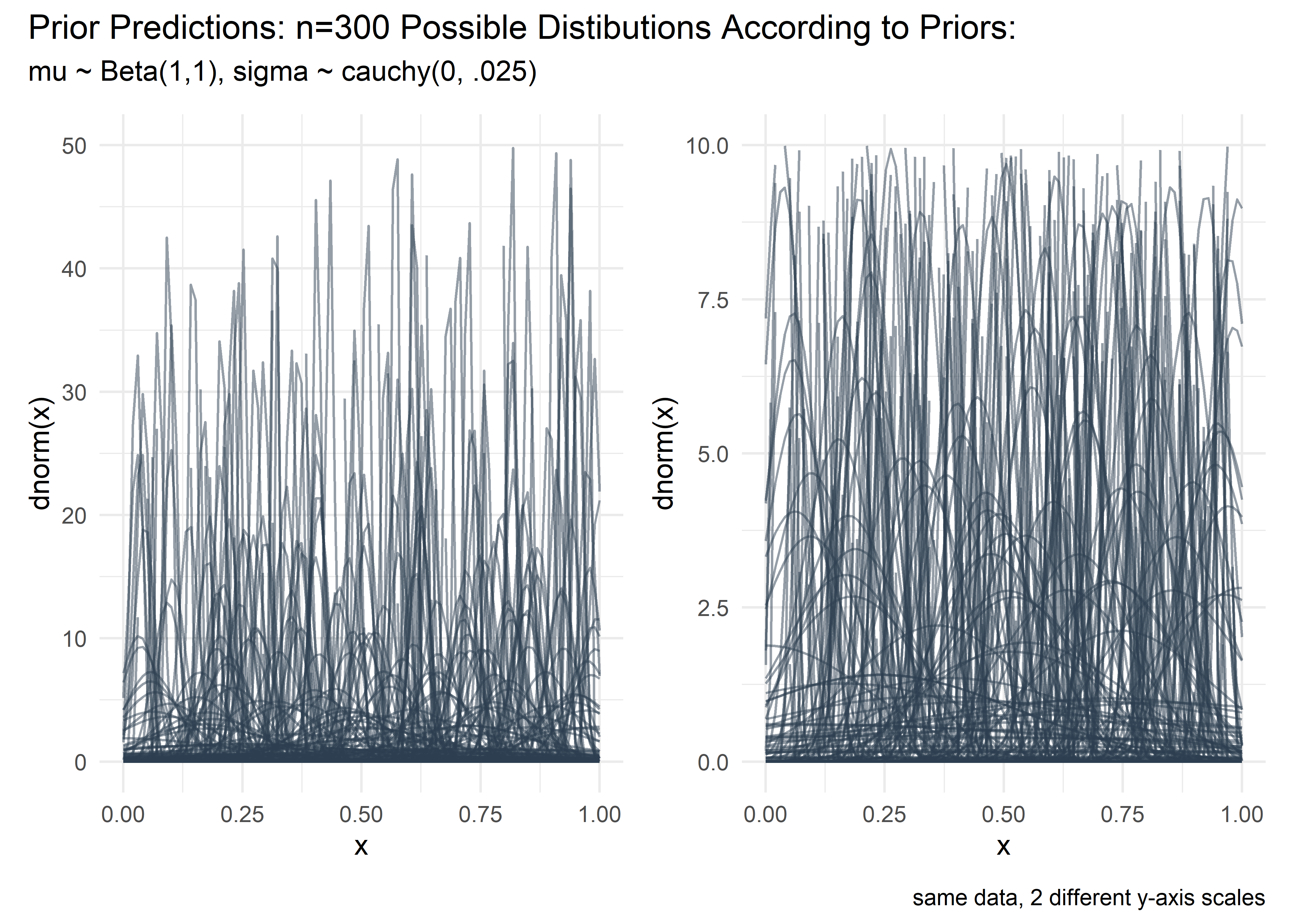
mutate(w_pct = w / 100)In preparation for the Bayesian tolerance interval calculations we should run some prior predictive checks. I know Beta(1,1) is a flat prior on mu, but I am not experienced enough with the cauchy to mentally visualize what its parameters mean with respect to the outcome variable. I adjusted the scale parameter for sigma manually and did this visual check each time until I saw a nice cloud of curves of varying but reasonable widths at scale = .025. Bonus - it is so satisfying to make the code for these curves using map2 and dplyr in the prep and then ggplot for the vis - incredibly smooth, readable, and efficient. I remain grateful for these core packages, especially as I start to mess around with other languages.
Prior Predictive Simulations
set.seed(2005)

prior_pred_tbl <- tibble(
  mu = rbeta(300, 1, 1),
  sig = rcauchy(300, 0, 0.025) %>% abs()
) %>%
  mutate(row_id = row_number()) %>%
  select(row_id, everything()) %>%
  mutate(plotted_y_data = map2(mu, sig, ~ tibble(
    x = seq(0, 1, length.out = 100),
    y = dnorm(x, .x, .y)
  ))) %>%
  unnest() %>%
  mutate(model = "mu ~ beta(1,1), sigma ~ cauchy(0,0.025)")

prior_pred_tbl %>%
gt_preview()| row_id | mu | sig | x | y | model | |
|---|---|---|---|---|---|---|
| 1 | 1 | 0.1675134 | 2.18178615 | 0.00000000 | 1.823131e-01 | mu ~ beta(1,1), sigma ~ cauchy(0,0.025) |
| 2 | 1 | 0.1675134 | 2.18178615 | 0.01010101 | 1.823759e-01 | mu ~ beta(1,1), sigma ~ cauchy(0,0.025) |
| 3 | 1 | 0.1675134 | 2.18178615 | 0.02020202 | 1.824349e-01 | mu ~ beta(1,1), sigma ~ cauchy(0,0.025) |
| 4 | 1 | 0.1675134 | 2.18178615 | 0.03030303 | 1.824900e-01 | mu ~ beta(1,1), sigma ~ cauchy(0,0.025) |
| 5 | 1 | 0.1675134 | 2.18178615 | 0.04040404 | 1.825412e-01 | mu ~ beta(1,1), sigma ~ cauchy(0,0.025) |
| 6..29999 | ||||||
| 30000 | 300 | 0.5856645 | 0.01596839 | 1.00000000 | 1.589627e-145 | mu ~ beta(1,1), sigma ~ cauchy(0,0.025) |
j <- prior_pred_tbl %>%
  ggplot(aes(x = x, y = y, group = row_id)) +
  geom_line(aes(x, y), alpha = .5, color = "#2c3e50") +
  labs(
    x = "x",
    y = "dnorm(x)"
  ) +
  ylim(c(0, 10)) +
  theme_minimal()

k <- j +
  ylim(c(0, 50))

(k + j) + plot_annotation(
  title = "Prior Predictions: n=300 Possible Distibutions According to Priors:",
  subtitle = "mu ~ Beta(1,1), sigma ~ cauchy(0, .025)",
  caption = "same data, 2 different y-axis scales"
)
Fit the model with brms
Use the priors that were just identified to fit a model in brms and visualize the output. The fuzzy caterpillar is not plotted because its very slow with to render with so many iterations. Don’t worry - it’s fuzzy.
Non-Informative Priors
w_mod <-
  brm(
    data = w_tbl, family = gaussian(),
    w_pct ~ 1,
    prior = c(
      prior(beta(1, 1), class = Intercept),
      prior(cauchy(0, .025), class = sigma)
    ),
    iter = 400000, warmup = 50000, chains = 4, cores = 2,
    seed = 10
  )


w_mod %>% summary()
## Family: gaussian
## Links: mu = identity; sigma = identity
## Formula: w_pct ~ 1
## Data: w_tbl (Number of observations: 16)
## Samples: 4 chains, each with iter = 4e+05; warmup = 50000; thin = 1;
## total post-warmup samples = 1400000
##
## Population-Level Effects:
## Estimate Est.Error l-95% CI u-95% CI Rhat Bulk_ESS Tail_ESS
## Intercept 0.67 0.00 0.67 0.67 1.00 858299 757467
##
## Family Specific Parameters:
## Estimate Est.Error l-95% CI u-95% CI Rhat Bulk_ESS Tail_ESS
## sigma 0.01 0.00 0.00 0.01 1.00 792388 740061
##
## Samples were drawn using sampling(NUTS). For each parameter, Bulk_ESS
## and Tail_ESS are effective sample size measures, and Rhat is the potential
## scale reduction factor on split chains (at convergence, Rhat = 1).Peek at the posterior tbl for mu and sigma.
w_post_tbl <-
  posterior_samples(w_mod) %>%
  select(-lp__) %>%
  rename("mu" = b_Intercept)

w_post_tbl %>%
gt_preview()| mu | sigma | |
|---|---|---|
| 1 | 0.6704184 | 0.004895014 |
| 2 | 0.6685570 | 0.005720891 |
| 3 | 0.6708761 | 0.003932762 |
| 4 | 0.6713238 | 0.004217306 |
| 5 | 0.6689520 | 0.005191162 |
| 6..1399999 | ||
| 1400000 | 0.6720105 | 0.005901202 |
Calculate 2-Sided Bayesian Tolerance Interval from the Posterior - Non-Informative Priors
Our goal is to calculate the 95/90 tolerance limit. The Bayesian analogue involves doing a row-wise calculation for each posterior draw where the equivalent of a tolerance interval is calculated using the standard formula: x +/- ks, where x is mu and s is sigma. The k factor is taken as the .95 quantile of a unit normal distribution (thus excluding the top and bottom 5% for 90% coverage). Doing this for every row in the posterior produces a distribution of upper and lower tolerance bounds - 1 observation for each credible set of mu and sigma. The 95% “confidence” analogue is done by excluding the 2.5% most extreme values from the low end of the lower bound distribution and the 2.5% most extreme values from the high end of the upper bound distribution.
bt_lower <- quantile(w_post_tbl$mu - qnorm(0.95) * w_post_tbl$sigma, 0.025)
bt_upper <- quantile(w_post_tbl$mu + qnorm(0.95) * w_post_tbl$sigma, 0.975)

bt_tbl <- tibble(
  lower_coverage_limit = bt_lower * 100 %>% round(4),
  upper_coverage_limit = bt_upper * 100 %>% round(4),
  method = as_factor("Bayesian")
)

bt_tbl %>%
gt_preview()| lower_coverage_limit | upper_coverage_limit | method | |
|---|---|---|---|
| 1 | 65.75688 | 68.44929 | Bayesian |
So the Bayesian version of a tolerance interval for those relatively vague priors is [65.84, 68.37] after back transforming the percentages to cg/g.
The frequentist version for the same data is calculated as follows with the tolerance package (assuming normality of the experimental data):
Frequentist 2-sided Tolerance Interval
fr_tbl <- tidy(normtol.int(w_tbl$w, alpha = .05, P = .9, side = 2, method = "EXACT")) %>%
  select(column, mean) %>%
  pivot_wider(
    names_from = "column",
    values_from = "mean"
  ) %>%
  select("2-sided.lower", "2-sided.upper") %>%
  mutate(method = as_factor("Frequentist")) %>%
  rename(
    lower_coverage_limit = "2-sided.lower",
    upper_coverage_limit = "2-sided.upper"
  ) %>%
  select(method, everything())
Combining and comparing to the Bayesian version:
fr_tbl %>%
  bind_rows(bt_tbl) %>%
  mutate_if(is.numeric, round, digits = 2) %>%
  mutate(priors = c("non_informative (implied)", "non-informative")) %>%
gt_preview()| method | lower_coverage_limit | upper_coverage_limit | priors | |
|---|---|---|---|---|
| 1 | Frequentist | 65.95 | 68.25 | non_informative (implied) |
| 2 | Bayesian | 65.76 | 68.45 | non-informative |
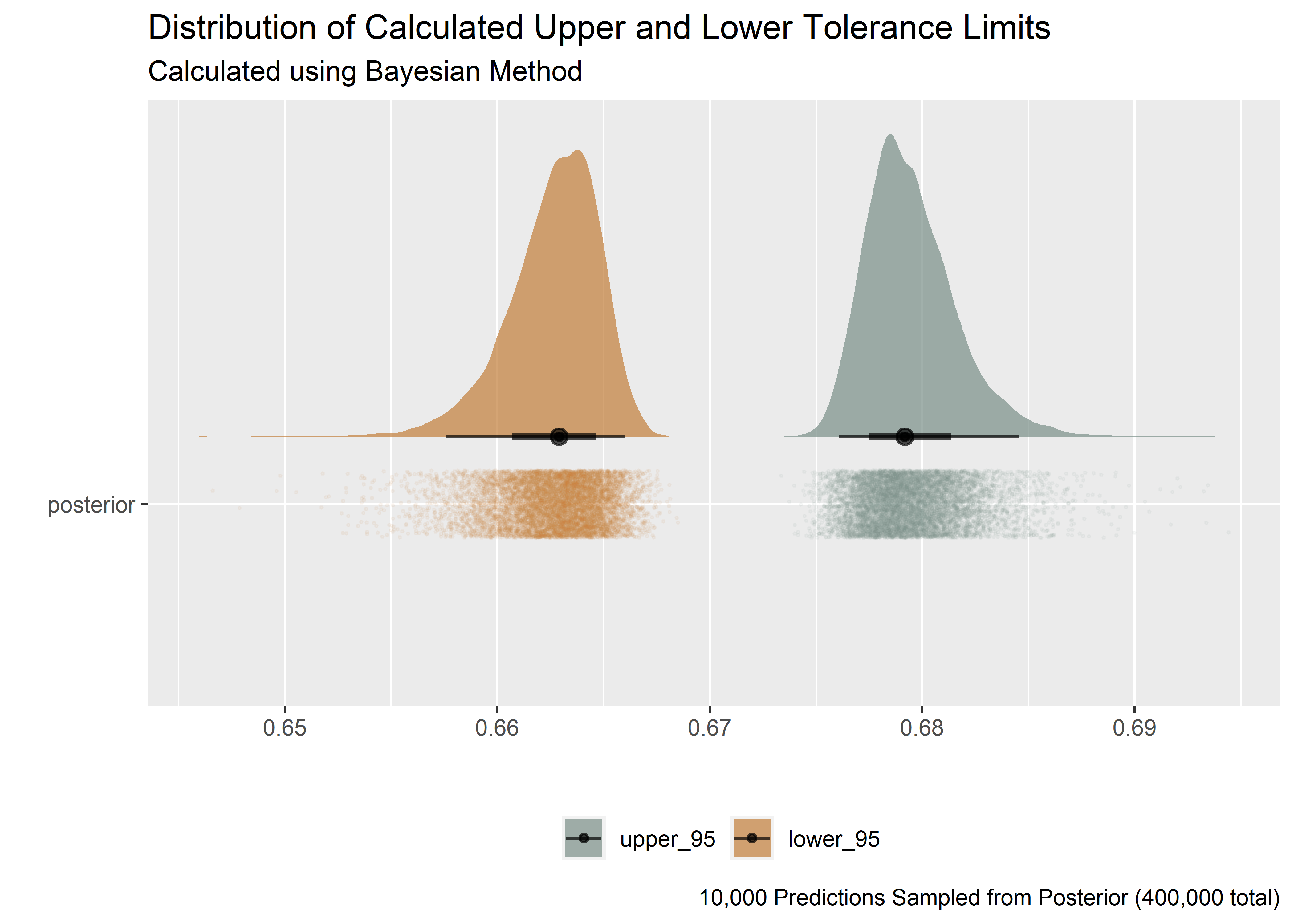
Plotting the upper and lower tolerance limits from the Bayesian version we see that the distribution (upper and lower bounds) are not normal.
w_post_tbl %>%
  mutate(
    upper_95 = qnorm(p = .95, mean = mu, sd = sigma),
    lower_95 = qnorm(p = .05, mean = mu, sd = sigma),
    id = as_factor("posterior")
  ) %>%
  sample_n(size = 10000) %>%
  pivot_longer(cols = c(upper_95, lower_95), names_to = "quantile", values_to = "value") %>%
  mutate(quantile = as_factor(quantile)) %>%
  ggplot(aes(x = value, y = id)) +
  geom_jitter(aes(color = quantile), width = .001, height = .1, size = .3, alpha = .05) +
  stat_halfeye(aes(fill = quantile), alpha = .7, position = position_nudge(y = .2)) +
  scale_color_manual(values = wes_palette("Moonrise2")) +
  scale_fill_manual(values = wes_palette("Moonrise2")) +
  #  scale_color_manual(values = c("purple", "limegreen")) +
  #  scale_fill_manual(values = c("purple", "limegreen")) +
  labs(
    x = "",
    y = "",
    title = "Distribution of Calculated Upper and Lower Tolerance Limits",
    subtitle = "Calculated using Bayesian Method",
    caption = "10,000 Predictions Sampled from Posterior (400,000 total)"
  ) +
  theme(
    legend.title = element_blank(),
    legend.position = "bottom"
  )
But the upper and lower bounds come in pairs. Plotting the pairs
set.seed(2345)

w_post_tbl %>%
  mutate(
    upper_95 = qnorm(p = .95, mean = mu, sd = sigma),
    lower_95 = qnorm(p = .05, mean = mu, sd = sigma)
  ) %>%
  sample_n(10000) %>%
  ggplot(aes(y = lower_95, x = upper_95)) +
  geom_point(alpha = .1, color = "#2c3e50") +
  geom_hline(yintercept = bt_lower, linetype = 2) +
  geom_vline(xintercept = bt_upper, linetype = 2) +
  theme_minimal() %>%
  labs(
    x = "Predicted upper tolerance bound",
    y = "Predicted lower tolerance bound",
    title = "Credible Values for Upper and Lower 95% Bounds",
    subtitle = "Based on Credible Posterior Draws",
    caption = "10,000 Predictions Sampled from Posterior (400,000 total)"
  )
Now we can calculate the number of tolerance bounds that are both:
- Above (within) the lower 95% tolerance bound for 90% coverage
- Below (within) the upper 95% tolerance bound for 90% coverage
This number should be less than 500 if the coverage interval is doing its job of capturing >= 95% of the credible range, since this is a subset of 10,000 draws from the full posterior (which wouldn’t display well).
set.seed(2345)

w_post_tbl %>%
  mutate(
    upper_95 = qnorm(p = .95, mean = mu, sd = sigma),
    lower_95 = qnorm(p = .05, mean = mu, sd = sigma)
  ) %>%
  sample_n(10000) %>%
  filter(
    lower_95 > bt_lower,
    upper_95 < bt_upper
  ) %>%
gt_preview()| mu | sigma | upper_95 | lower_95 | |
|---|---|---|---|---|
| 1 | 0.6734567 | 0.005124883 | 0.6818864 | 0.6650271 |
| 2 | 0.6705619 | 0.004108660 | 0.6773200 | 0.6638037 |
| 3 | 0.6704661 | 0.005681679 | 0.6798116 | 0.6611206 |
| 4 | 0.6709579 | 0.003404294 | 0.6765575 | 0.6653584 |
| 5 | 0.6706663 | 0.004703547 | 0.6784029 | 0.6629296 |
| 6..9541 | ||||
| 9542 | 0.6713993 | 0.004295096 | 0.6784641 | 0.6643345 |
If you’ve made it this far, thank you for your attention.
Session Info
sessionInfo()## R version 4.0.3 (2020-10-10)
## Platform: x86_64-w64-mingw32/x64 (64-bit)
## Running under: Windows 10 x64 (build 18363)
##
## Matrix products: default
##
## locale:
## [1] LC_COLLATE=English_United States.1252
## [2] LC_CTYPE=English_United States.1252
## [3] LC_MONETARY=English_United States.1252
## [4] LC_NUMERIC=C
## [5] LC_TIME=English_United States.1252
##
## attached base packages:
## [1] stats graphics grDevices utils datasets methods base
##
## other attached packages:
## [1] gt_0.2.2 patchwork_1.1.0 wesanderson_0.3.6 tolerance_2.0.0
## [5] tidybayes_2.3.1 broom_0.7.2 brms_2.14.4 Rcpp_1.0.5
## [9] here_1.0.0 forcats_0.5.0 stringr_1.4.0 dplyr_1.0.2
## [13] purrr_0.3.4 readr_1.4.0 tidyr_1.1.2 tibble_3.0.4
## [17] ggplot2_3.3.2 tidyverse_1.3.0
##
## loaded via a namespace (and not attached):
## [1] readxl_1.3.1 backports_1.2.0 plyr_1.8.6
## [4] igraph_1.2.6 splines_4.0.3 svUnit_1.0.3
## [7] crosstalk_1.1.0.1 rstantools_2.1.1 inline_0.3.16
## [10] digest_0.6.27 htmltools_0.5.0 rsconnect_0.8.16
## [13] fansi_0.4.1 checkmate_2.0.0 magrittr_2.0.1
## [16] modelr_0.1.8 RcppParallel_5.0.2 matrixStats_0.57.0
## [19] xts_0.12.1 prettyunits_1.1.1 colorspace_2.0-0
## [22] rvest_0.3.6 ggdist_2.3.0 haven_2.3.1
## [25] xfun_0.19 callr_3.5.1 crayon_1.3.4
## [28] jsonlite_1.7.1 lme4_1.1-25 zoo_1.8-8
## [31] glue_1.4.2 gtable_0.3.0 emmeans_1.5.2-1
## [34] webshot_0.5.2 V8_3.4.0 distributional_0.2.1
## [37] pkgbuild_1.1.0 rstan_2.21.2 abind_1.4-5
## [40] scales_1.1.1 mvtnorm_1.1-1 DBI_1.1.0
## [43] miniUI_0.1.1.1 xtable_1.8-4 stats4_4.0.3
## [46] StanHeaders_2.21.0-6 DT_0.16 htmlwidgets_1.5.2
## [49] httr_1.4.2 threejs_0.3.3 arrayhelpers_1.1-0
## [52] ellipsis_0.3.1 farver_2.0.3 pkgconfig_2.0.3
## [55] loo_2.3.1 sass_0.3.1 dbplyr_2.0.0
## [58] labeling_0.4.2 manipulateWidget_0.10.1 tidyselect_1.1.0
## [61] rlang_0.4.9 reshape2_1.4.4 later_1.1.0.1
## [64] munsell_0.5.0 cellranger_1.1.0 tools_4.0.3
## [67] cli_2.2.0 generics_0.1.0 ggridges_0.5.2
## [70] evaluate_0.14 fastmap_1.0.1 yaml_2.2.1
## [73] processx_3.4.4 knitr_1.30 fs_1.5.0
## [76] rgl_0.103.5 nlme_3.1-150 mime_0.9
## [79] projpred_2.0.2 xml2_1.3.2 compiler_4.0.3
## [82] bayesplot_1.7.2 shinythemes_1.1.2 rstudioapi_0.13
## [85] gamm4_0.2-6 curl_4.3 reprex_0.3.0
## [88] statmod_1.4.35 stringi_1.5.3 ps_1.4.0
## [91] blogdown_0.15 Brobdingnag_1.2-6 lattice_0.20-41
## [94] Matrix_1.2-18 nloptr_1.2.2.2 markdown_1.1
## [97] shinyjs_2.0.0 vctrs_0.3.5 pillar_1.4.7
## [100] lifecycle_0.2.0 bridgesampling_1.0-0 estimability_1.3
## [103] httpuv_1.5.4 R6_2.5.0 bookdown_0.21
## [106] promises_1.1.1 gridExtra_2.3 codetools_0.2-18
## [109] boot_1.3-25 colourpicker_1.1.0 MASS_7.3-53
## [112] gtools_3.8.2 assertthat_0.2.1 rprojroot_2.0.2
## [115] withr_2.3.0 shinystan_2.5.0 mgcv_1.8-33
## [118] parallel_4.0.3 hms_0.5.3 grid_4.0.3
## [121] coda_0.19-4 minqa_1.2.4 rmarkdown_2.5
## [124] shiny_1.5.0 lubridate_1.7.9.2 base64enc_0.1-3
## [127] dygraphs_1.1.1.6Stoudt S, Pintar A, Possolo A (2021) Coverage Intervals. J Res Natl Inst Stan 126:126004. https://doi.org/10.6028/jres.126.004. ↩︎