Learning from Failure - Nitinol Fracture Mechanics in R

Initial Crack Size and Crack Growth Rate

Here is our toy fracture surface.¹

Let \(a\) equal the crack length (inclusion size) -> 2.0 um.

a <- 2E-6 # units: meters

Now we zoom in and measure the spacing of the fatigue striations.²

Let \(da \over dN\) equal the crack growth rate (striation width) -> .007 um

da_dn <- 7E-9

Paris’ Law

Paris’ Law gives the relationship between crack growth rate and stress intensity range \(\Delta K\) during the period of constant crack growth. We actually want strain amplitude, but \(\Delta K\) is an intermediate that we have to think about first.

\[{da \over dN}=C(\Delta K)^{m}\] On a log scale, this equation is a line where \(m\) is the slope, \(C\) is the y-intercept constant, \(\Delta K\) is the predictor variable, and \(da \over dN\) is the response variable. For nitinol and many other engineering materials, benevolent engineers have painstakingly established these parameters and shared them in literature for a variety of loading ratios. The fitted parameters can also be visually confirmed against the reference data using plots like below.³

Using the average reported for Load Ratios R = 0.1 and R = 0.5:

Let \(m\) equal the slope -> 3.82

Let \(C\) equal the intercept -> 1.574e-10

m <- 3.82 # units: (m/cycle) / (MPa * m^.5)
c <- 1.574e-10 # units: m/cycle

Rearranging and solving for \(\Delta K\):

#  da_dn <- c*(k^m)
#  da_dn/c <- k^m
delta_k <- (da_dn / c)^(1 / m) # MPa*sqrt(m)

From Stress Intensity to Stress

Now we have a stress intensity range but we want strain amplitude. By definition, the magnitude of \(\Delta K\) depends on specimen geometry, size and location of crack, and magnitude of alternating stress. This where our measurement of inclusion size at crack origin \(a\) in comes in (note: geometry factor of 0.65 taken from literature):⁴

\[{\Delta K=0.65\Delta \sigma {\sqrt {\pi a}}}\]

Stress Range to Strain Amplitude

We also know that stress is related to strain via Hooke’s Law, so we need a material property for austenite modulus \(E\).⁵ These are easy to find or measure; we’ll use 66,000 MPa.

E <- 66000 # units: MPa

Now we have everything we need to find the strain amplitude. Note that the strain amplitude will be half the strain range.

# delta_k = 0.65 * delta_stress * (pi * a)^.5
# delta_stress <- delta_k * (1/0.65) / (pi * a)^.5

delta_strain <- (1 / E) * delta_k * (1 / 0.65) / (pi * a)^.5 # this is peak-to-peak strain amp or strain range
strain_amp <- delta_strain / 2

strain_amp

## [1] 0.01255627

To sum it up and make it easier next time: here is the full expression that gets you from the observed features of the fracture to the desired strain amplitude in 1 go (using all the assumptions previously stated):

strain_amp <- (0.7692308 / E) * (da_dn / c)^(1 / m) / (pi * a)^.5
strain_amp

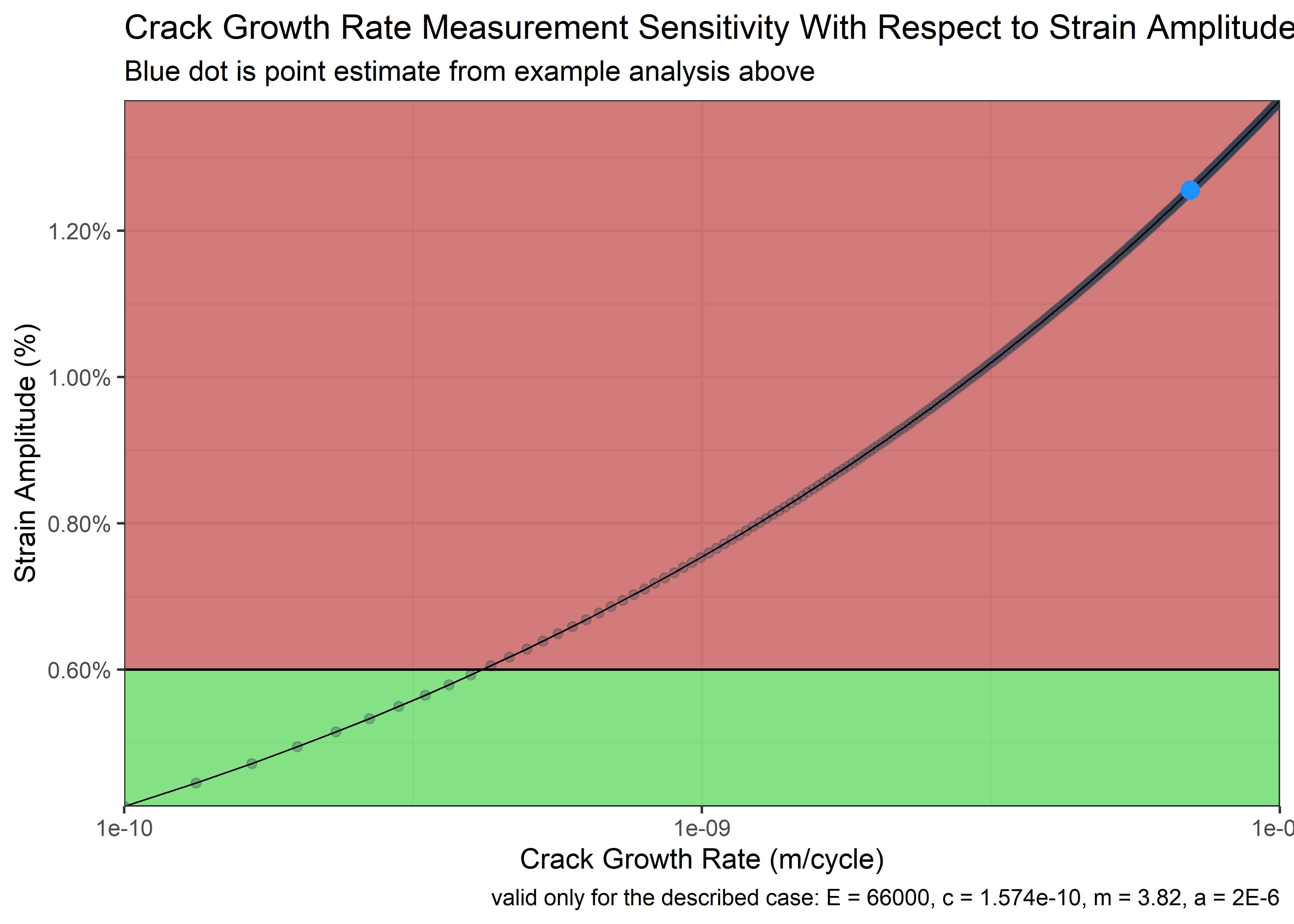
## [1] 0.01255628

So we have an estimated strain amplitude of 1.3%! This value passes the gut check because nitinol tends to fracture in the 0.2 - 0.7% range, depending on a variety of other factors like mean strain, compression strain, strain volume, etc. So no surprise that it fractured - but we could compare this number against our predictive FEA and try to figure out if our boundary conditions are reasonable for modeling or perhaps we missed on one of our modeling assumptions.

Strain Amp Function

sens_fct <- function(dadn, E = 66000, c = 1.574e-10, m = 3.82, a = 2E-6) {
  de <- (0.7692308 / E) * (dadn / c)^(1 / m) / (pi * a)^.5
  return(de)
}

Map the Function Over Some Inputs

First, we setup a sequence of crack growth rates that might represent a reasonable range given the measurement error of striations on our fracture surface. The range covers 2 orders of magnitude. Then, we map the strain function over the inputs.

sens_tbl <- tibble(dadn = seq(from = 1E-10, to = 1E-8, length.out = 300)) %>%
  mutate(strain_amp = map_dbl(.x = dadn, .f = sens_fct))

sens_tbl

## # A tibble: 300 x 2
##        dadn strain_amp
##       <dbl>      <dbl>
##  1 1   e-10    0.00413
##  2 1.33e-10    0.00445
##  3 1.66e-10    0.00472
##  4 1.99e-10    0.00495
##  5 2.32e-10    0.00515
##  6 2.66e-10    0.00533
##  7 2.99e-10    0.00550
##  8 3.32e-10    0.00565
##  9 3.65e-10    0.00579
## 10 3.98e-10    0.00593
## # ... with 290 more rows

Visualize

The plot below shows the sensitivity to crack growth rate measurement accuracy. The red dot represents our point estimate from the work above. A reference line at 0.6% is added to represent and approximate threshold where we might start to believe the implant should have survived. There’s a little vis trick here where you have to feed geom_rect() a 1 line dummy dataframe to get the alpha transparency down.

sens_plt <- sens_tbl %>%
  ggplot(aes(x = dadn, y = strain_amp)) +
  geom_rect(data = sens_tbl[1, ], aes(xmin = min(sens_tbl$dadn), xmax = max(sens_tbl$dadn), ymin = min(sens_tbl$strain_amp), ymax = .006), alpha = .6, fill = "limegreen") +
  geom_rect(data = sens_tbl[1, ], aes(xmin = min(sens_tbl$dadn), xmax = max(sens_tbl$dadn), ymin = .006, ymax = max(sens_tbl$strain_amp)), alpha = .6, fill = "firebrick") +
  geom_point(alpha = .3, color = "#2c3e50") +
  geom_line(size = .3) +
  geom_point(data = tibble(dadn = 7E-9, strain_amp = 0.01255628), color = "dodgerblue", size = 3) +
  geom_hline(aes(yintercept = .006)) +
  theme_bw() +
  labs(
    x = "Crack Growth Rate (m/cycle)",
    y = "Strain Amplitude (%)",
    title = "Crack Growth Rate Measurement Sensitivity With Respect to Strain Amplitude",
    subtitle = "Blue dot is point estimate from example analysis above",
    caption = "valid only for the described case: E = 66000, c = 1.574e-10, m = 3.82, a = 2E-6"
  ) +
  scale_x_continuous(expand = c(0, 0), trans = "log10") +
  scale_y_continuous(expand = c(0, 0), labels = scales::percent)

sens_plt

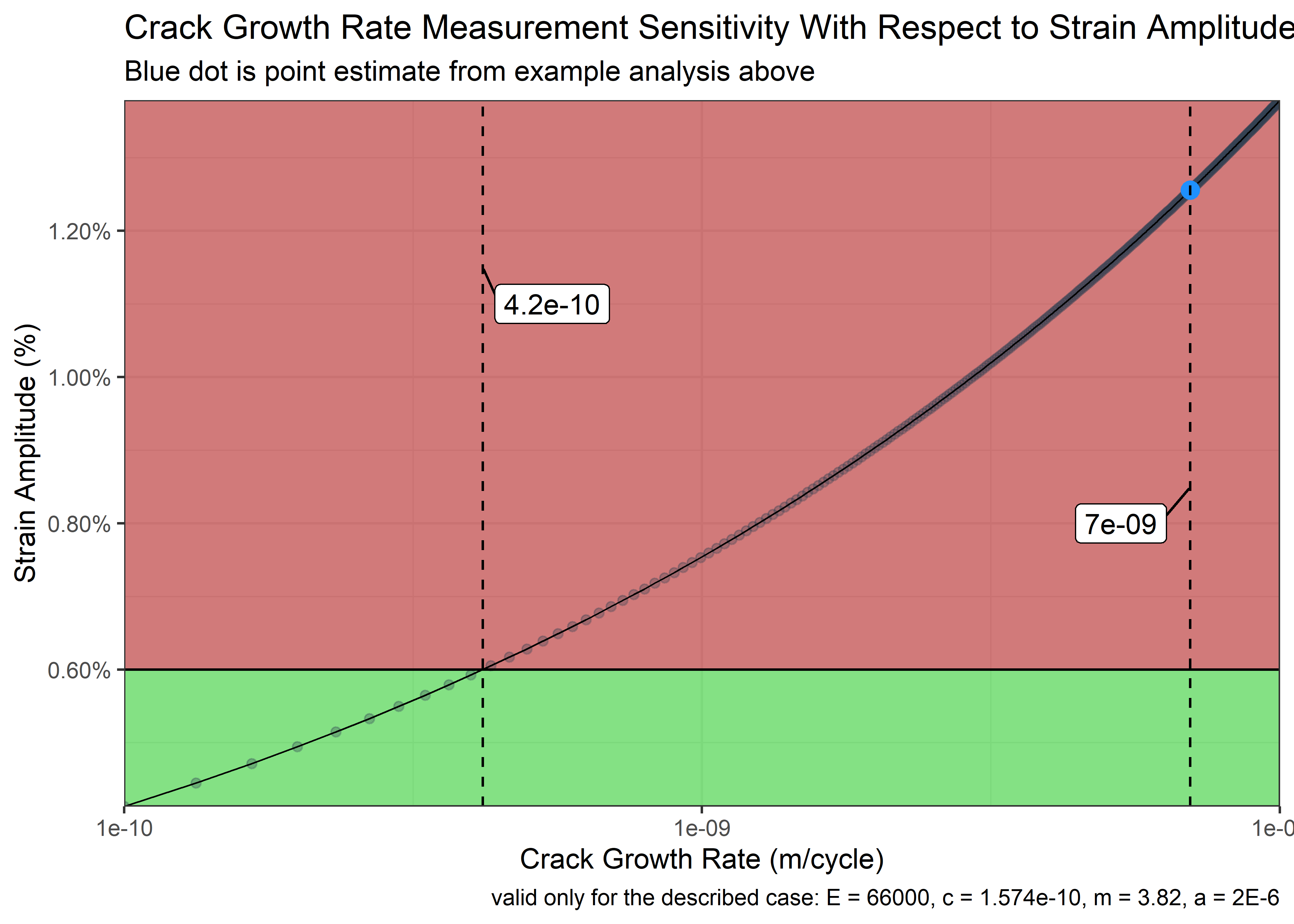
Just for fun and practice, we could identify that point where the function intersects the .6% decision line. First, we modify our function slightly to return the distance from the function to the reference line.

sens_min_fcn <- function(dadn, E = 66000, c = 1.574e-10, m = 3.82, a = 2E-6) {
  de <- ((0.7692308 / E) * (dadn / c)^(1 / m) / (pi * a)^.5) - .006
  return(de)
}

Now, we utilize the uniroot function to zero find. This function does not minimize - it looks for a zero. So we need an interval for which the function would return a negative number on one end and a positive on the other (bounding the zero target).

root <- uniroot(f = sens_min_fcn, interval = c(1e-10, 1e-8), tol = 1E-11)
root

## $root
## [1] 4.175116e-10
## 
## $f.root
## [1] 2.463828e-06
## 
## $iter
## [1] 5
## 
## $init.it
## [1] NA
## 
## $estim.prec
## [1] 6.70181e-12

Confirming visually:

sens_plt +
  geom_vline(aes(xintercept = root$root), linetype = 2) +
  geom_vline(aes(xintercept = 7E-9), linetype = 2) +
  geom_label_repel(
    data = tibble(dadn = root$root, strain_amp = .0115, label = str_glue({
      root$root %>% round(digits = 11)
    })),
    aes(label = label), min.segment.length = .05, nudge_x = .12, nudge_y = -.0005
  ) +
  geom_label_repel(
    data = tibble(dadn = 7.0E-9, strain_amp = .0085, label = round(7.0E-9, digits = 11)),
    aes(label = label), min.segment.length = .05, nudge_x = -.12, nudge_y = -.0005
  )

The measurement error necessary to move us all the way to that .6% decision boundary is therefore:

7E-9 - 4.2E-10

## [1] 6.58e-09