Suppose our team is preparing to freeze a new implant design. In order to move into the next phase of the PDP, it is common to perform a suite of formal “Design Freeze” testing. If the results of the Design Freeze testing are acceptable, the project can advance from Design Freeze (DF) into Design Verification (DV). DV is an expensive and resource intensive phase culminating in formal reports that are included in the regulatory submission. One key goal of DF is therefore to burn down enough risk to feel confident going into DV. Despite the high stakes, I haven’t ever seen a quantitative assessment of residual risk at the phase review. In this post we’ll attempt to use some simple Bayesian methods to quantify the DV risk as a function of DF sample size for a single, high-risk test.
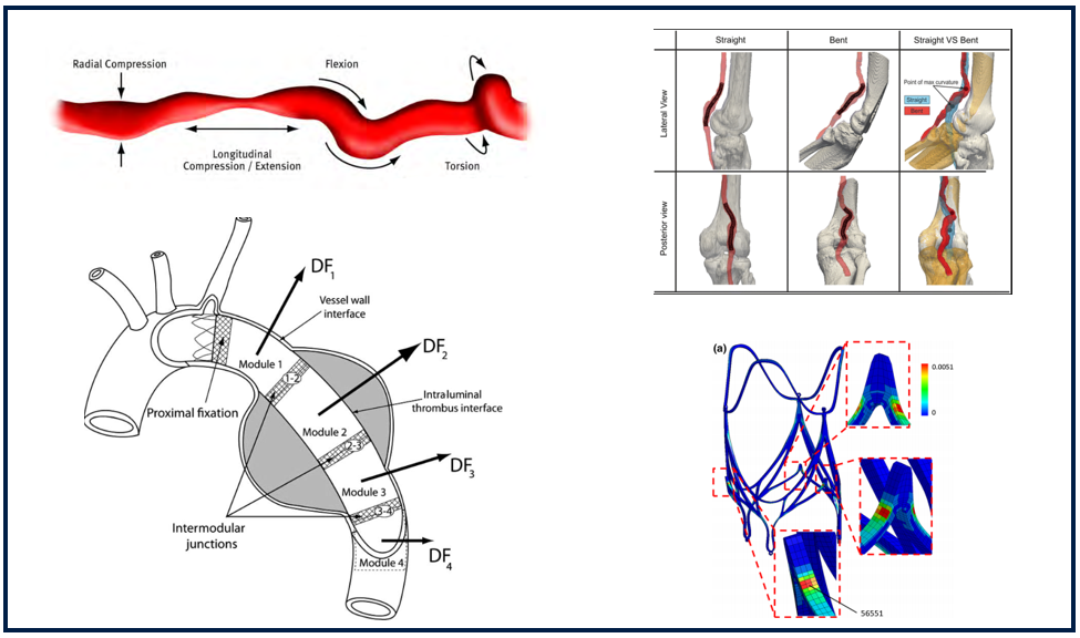
Consider the requirement for accelerated durability (sometimes called fatigue resistance). In this test, the device is subjected to cyclic loading for a number of cycles equal to the desired service life. For 10 years of loading due to systolic - diastolic pressure cycles, vascular implants must survive approximately 400 million cycles. Accelerated durability is usually treated as attribute type data because the results can be only pass (if no fractures observed) or fail (if fractures are observed). Each test specimen can therefore be considered a Bernoulli trial and the number of passing units in n samples can be modeled with the binomial.
How many samples should we include in DF? We’ll set up some simulations to find out. In order to incorporate the outcome of the DF data into a statement about the probability of success for DV, we’ll need to apply Bayesian methods.
First, load the libraries:
library(tidyverse)
library(cowplot)
library(gghighlight)
library(knitr)
library(kableExtra)
The simulation should start off before we even execute Design Freeze testing. If we’re going to use Bayesian techniques we need to express our uncertainty about the parameters in terms of probability. In this case, the parameter we care about is the reliability. Before seeing any DF data we might know very little about what the true reliability is for this design. If we were asked to indicate what we thought the reliability might be, we should probably state a wide range of possibilities. The design might be good but it might be quite poor. Our belief about the reliability before we do any testing at all is called the prior and we expess it as a probability density function, not a point estimate. We need a mathematical function to describe how we want to spread out our belief in the true reliability.
The beta is a flexible distribution that can be adjusted to take a variety of different forms. By tweaking the two shape factors of the beta we can customize the probability density curve in many different ways. If we were super confident that every part we ever made would pass the durability testing, we could put a “spike” prior right on 1.0. This is like saying “there’s no way any part could ever fail”. But the whole point is to communicate uncertainty and in reality there is always a chance the reliability might only be 97%, or 94%, etc. Since we haven’t really seen any DF data, we should probably drop some of our credibility into many different possible values of the reliability. Let’s be very conservative here and just use the flat prior. By evenly binning all of our credibility across the full range of reliability from 0 to 1, we’re saying we don’t want our pre-conceived notions to influence the final estimated reliability much. We’ll instead use the DF data themselves to re-allocate the credibility across the range of reliabilities appropriately according to Bayes’ rule after looking at the Design Freeze results. The more DF data we observe, the more precise the posterior estimate.
The mathematical way to turn the beta distribution into a straight line (flat prior) is to set the shape parameters alpha and beta to (1,1). Note the area under the curve must always sum to 1. The image on the left shows a flat prior generated from a beta density with parameters (1,1).
Another way to display the prior is to build out the visualization manually by drawing random values from the beta(1,1) distribution and constructing a histogram. This method isn’t terribly useful since we already know the exact distribution we want to use but I like to include it to emphasize the idea of “binning” the credibility across different values of reliability. It’s also nice to see the uncertainty we might see when we start to randomly draw from the distribution (full disclosure: I also just to practice my coding).
#Plot flat prior using stat_function and ggplot
p_1 <- tibble(x_canvas=c(0,1)) %>% ggplot(aes(x=x_canvas)) +
    stat_function(fun   = dbeta,
                  args  = list(1, 1),
                  color = "#2c3e50",
                  size  = 1,
                  alpha = .8) +
    ylim(c(0,1.5)) +
    labs(
        y = "Density of Beta",
        x = "Reliability",
        title = "Credibility Allocation, Start of DF",
        subtitle = "Uninformed Prior with Beta (1,1)"
    )

#Set the number of random draws from beta(1,1) to construct histogram flat prior
set.seed(123)
n_draws <- 100000

#Draw random values from beta(1,1), store in object
prior_dist_sim <- rbeta(n = n_draws, shape1 = 1, shape2 = 1)

#Convert from vector to tibble
prior_dist_sim_tbl <- prior_dist_sim %>% as_tibble()

#Visualize with ggplot
p_2 <- prior_dist_sim_tbl %>% ggplot(aes(x = value)) +
    geom_histogram(
        boundary = 1,
        binwidth = .05,
        color    = "white",
        fill     = "#2c3e50",
        alpha    = 0.8
        ) +
    xlim(c(-0.05, 1.05)) +
    ylim(c(0, 7500)) +
    labs(
        y = "Count",
        title = "Credibility Simulation , Start of DF",
        subtitle = "Uninformed Prior with Beta (1,1)",
        x = "Reliability"

    )

plot_grid(p_1,p_2)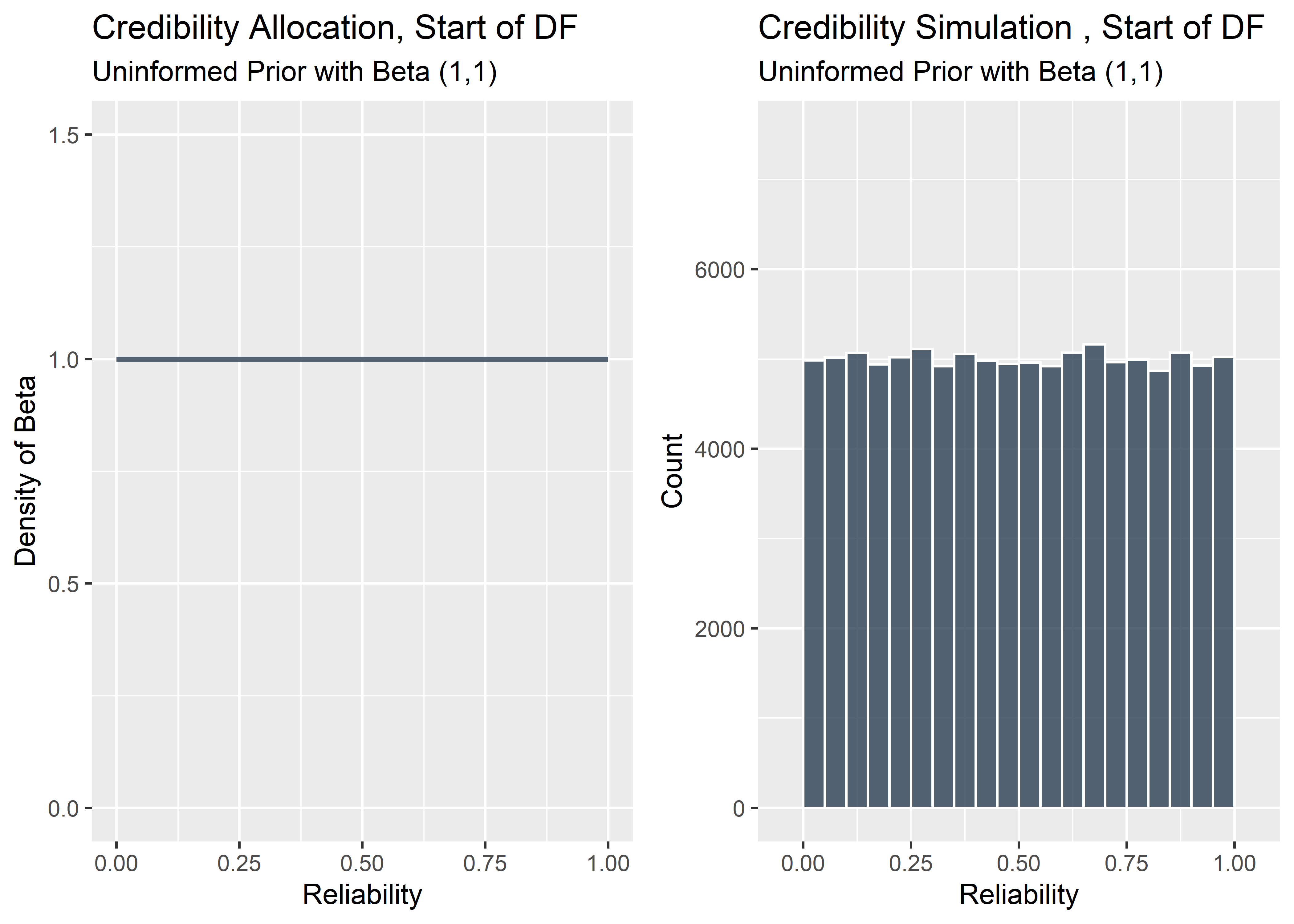
OK now the fun stuff. There is a cool, mathematical shortcut we can take to combine our simulated Design Freeze data with our flat prior to create the posterior distribution. It’s very simple: we just add the number of passing DF units to our alpha parameter and the number of failing DF units to our beta parameter. The reason why this works so well is beyond the scope of this post, but the main idea is that when the functional form of the prior (beta function in our case) is similar to the functional form of the likelihood function (Bernoulli in our case), then you can multiply them together easily and the product also takes a similar form. When this happens, the prior is said to be the “conjugate prior” of the likelihood function 1 The beta and binomial are a special case that go together like peanut butter and jelly.
Again, to understand how our belief in the reliability should be allocated after observing the DF data, all we need to do is update the beta function by adding the number of passing units from DF testing to alpha (Shape1 parameter) and the number of failing units to beta (Shape2 parameter).
\[\mbox{Beta}(\alpha_0+\mbox{passes}, \beta_0+\mbox{fails})\] We’re going to assume all units pass DF, so we only need to adjust the alpha parameter. The resulting beta distribution that we get after updating the alpha parameter represents our belief in where the true reliability may lie after observing the DF data. Remember, even though every unit passed, we can’t just say the reliability is 100% because we’re smart enough to know that if the sample size was, for example, n=15 - there is a reasonable chance that a product with true reliability of 97% could run off n=15 in a row without failing. Even 90% reliability might hit 15 straight every once in a while but it would be pretty unlikely.
The code below looks at four different possible sample size options for DF: n=15, n=30, n=45, and a full n=59 (just like we plan for DV).
#Draw radomly from 4 different beta distributions. Alpha parameter is adjusted based on DF sample size
posterior_dist_sim_15 <- rbeta(n_draws, 16, 1)
posterior_dist_sim_30 <- rbeta(n_draws, 31, 1)
posterior_dist_sim_45 <- rbeta(n_draws, 46, 1)
posterior_dist_sim_59 <- rbeta(n_draws, 60, 1)

#Function to convert vectors above into tibbles and add column for Sample Size
pds_clean_fcn <- function(pds, s_size){
    pds %>% as_tibble() %>% mutate(Sample_Size = s_size) %>%
    mutate(Sample_Size = factor(Sample_Size, levels = unique(Sample_Size)))}

#Apply function to 4 vectors above
posterior_dist_sim_15_tbl <- pds_clean_fcn(posterior_dist_sim_15, 15)
posterior_dist_sim_30_tbl <- pds_clean_fcn(posterior_dist_sim_30, 30)
posterior_dist_sim_45_tbl <- pds_clean_fcn(posterior_dist_sim_45, 45)
posterior_dist_sim_59_tbl <- pds_clean_fcn(posterior_dist_sim_59, 59)

#Combine the tibbles in a tidy format for visualization
full_post_df_tbl <- bind_rows(
            posterior_dist_sim_15_tbl,
            posterior_dist_sim_30_tbl,
            posterior_dist_sim_45_tbl,
            posterior_dist_sim_59_tbl
            )

#Visualize with density plot
df_density_plt <- full_post_df_tbl %>% ggplot(aes(x = value, fill = Sample_Size)) +
    geom_density(alpha = .6) +
    xlim(c(0.85,1)) +
    labs(x = "",
         y = "Density of Beta",
         title = "Credibility Simulation, After Design Freeze",
         subtitle = "Updated Belief Modeled with Beta(1 + n,1)") +
    scale_fill_manual(values = c("#2C728EFF", "#20A486FF", "#75D054FF", "#FDE725FF"))

#Visualize with histogram
df_hist_plt <- full_post_df_tbl %>% ggplot(aes(x = value, fill = Sample_Size)) +
    geom_histogram(alpha = .9,
                   position = "dodge",
                   boundary = 1,
                   color = "black") +
    xlim(c(0.85,1)) +
    labs(x = "Reliability",
         y = "Count") +
    scale_fill_manual(values = c("#2C728EFF", "#20A486FF", "#75D054FF", "#FDE725FF"))

plot_grid(df_density_plt, df_hist_plt, ncol = 1)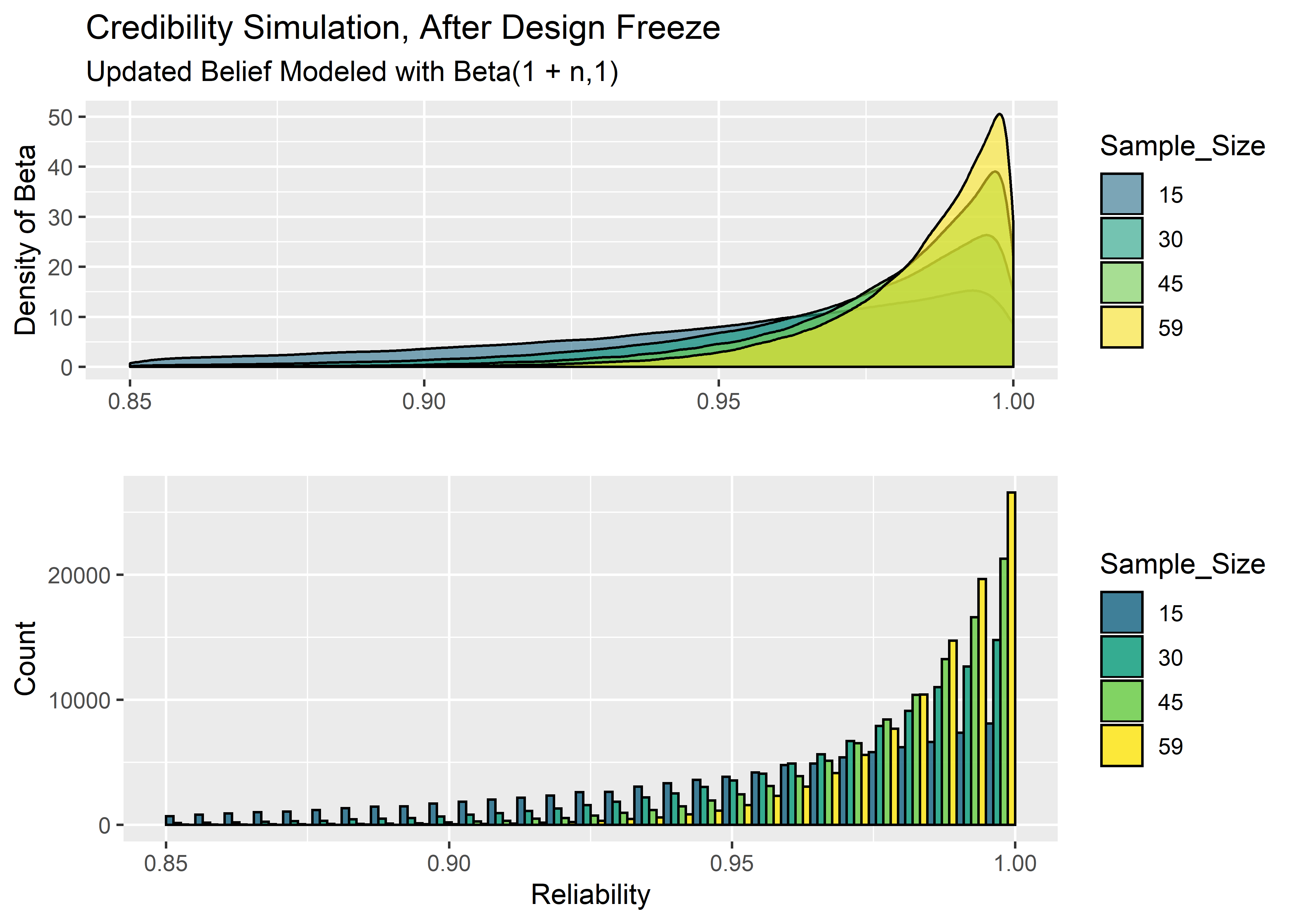
If we unpack these charts a bit, we can see that if we only do n=15 in Design Freeze, we still need to allocate some credibility to reliability parameters below .90. For a full n=59, anything below .95 reliability is very unlikely, yet the 59 straight passing units could have very well come from a product with reliability = .98 or .97.
We now have a good feel for our uncertainty about the reliability after DF, but what we really want to know is our likelihood of passing Design Verification. To answer this question, we’ll extend our simulation to perform many replicates of n=59 Bernoulli trials, each representing a round of Design Verification testing. The probability of failure will be randomly drawn from the distributions via Monte Carlo. Let’s see how many of these virtual DV tests end with 59/59 passing:
#Perform many sets of random binom runs, each with n=59 trials. p is taken from the probs previously generated
DV_acceptable_units_15 <- rbinom(size = 59, n = n_draws,
                                 prob = (posterior_dist_sim_15_tbl$value))
DV_acceptable_units_30 <- rbinom(size = 59, n = n_draws,
                                 prob = (posterior_dist_sim_30_tbl$value))
DV_acceptable_units_45 <- rbinom(size = 59, n = n_draws,
                                 prob = (posterior_dist_sim_45_tbl$value))
DV_acceptable_units_59 <- rbinom(size = 59, n = n_draws,
                                 prob = (posterior_dist_sim_59_tbl$value))

#Function to convert vectors to tibbles and add col for sample size
setup_fcn <- function(vec, ss){
    vec %>% as_tibble() %>% mutate(DF_Sample_Size = ss) %>%
    mutate(DF_Sample_Size = factor(DF_Sample_Size, levels = unique(DF_Sample_Size)))}

#Apply function
DV_acceptable_units_15_tbl <- setup_fcn(DV_acceptable_units_15, 15)
DV_acceptable_units_30_tbl <- setup_fcn(DV_acceptable_units_30, 30)
DV_acceptable_units_45_tbl <- setup_fcn(DV_acceptable_units_45, 45)
DV_acceptable_units_59_tbl <- setup_fcn(DV_acceptable_units_59, 59)

#Combine the tibbles in a tidy format for visualization
DV_acceptable_full_tbl <- bind_rows(DV_acceptable_units_15_tbl,
                                    DV_acceptable_units_30_tbl,
                                    DV_acceptable_units_45_tbl,
                                    DV_acceptable_units_59_tbl)

#Visualize with ggplot.  Apply gghighlight where appropriate
g1 <- DV_acceptable_full_tbl %>%
   ggplot(aes(x = value)) +
   geom_histogram(aes(fill = DF_Sample_Size),binwidth = 1, color = "black", position = "dodge", alpha = .9) +
    xlim(c(45, 60)) +
    scale_x_continuous(limits = c(45, 60), breaks=seq(45, 60, 1)) +
    scale_fill_manual(values = c("#2C728EFF", "#20A486FF", "#75D054FF", "#FDE725FF")) +
    labs(
        x = "Passing Parts out of 59 total",
        title = "Simulated Design Verification Testing",
        subtitle = "100,000 Simulated DV Runs of n=59"
    )

g2 <- g1 +
    gghighlight(value == 59, use_direct_label = FALSE) +
    labs(
        title = "Simulations that PASSED Design Verification"
     )

g3 <- g1 +
    gghighlight(value < 59, use_direct_label = FALSE) +
    labs(
        title = "Simulations that FAILED Design Verification"
    )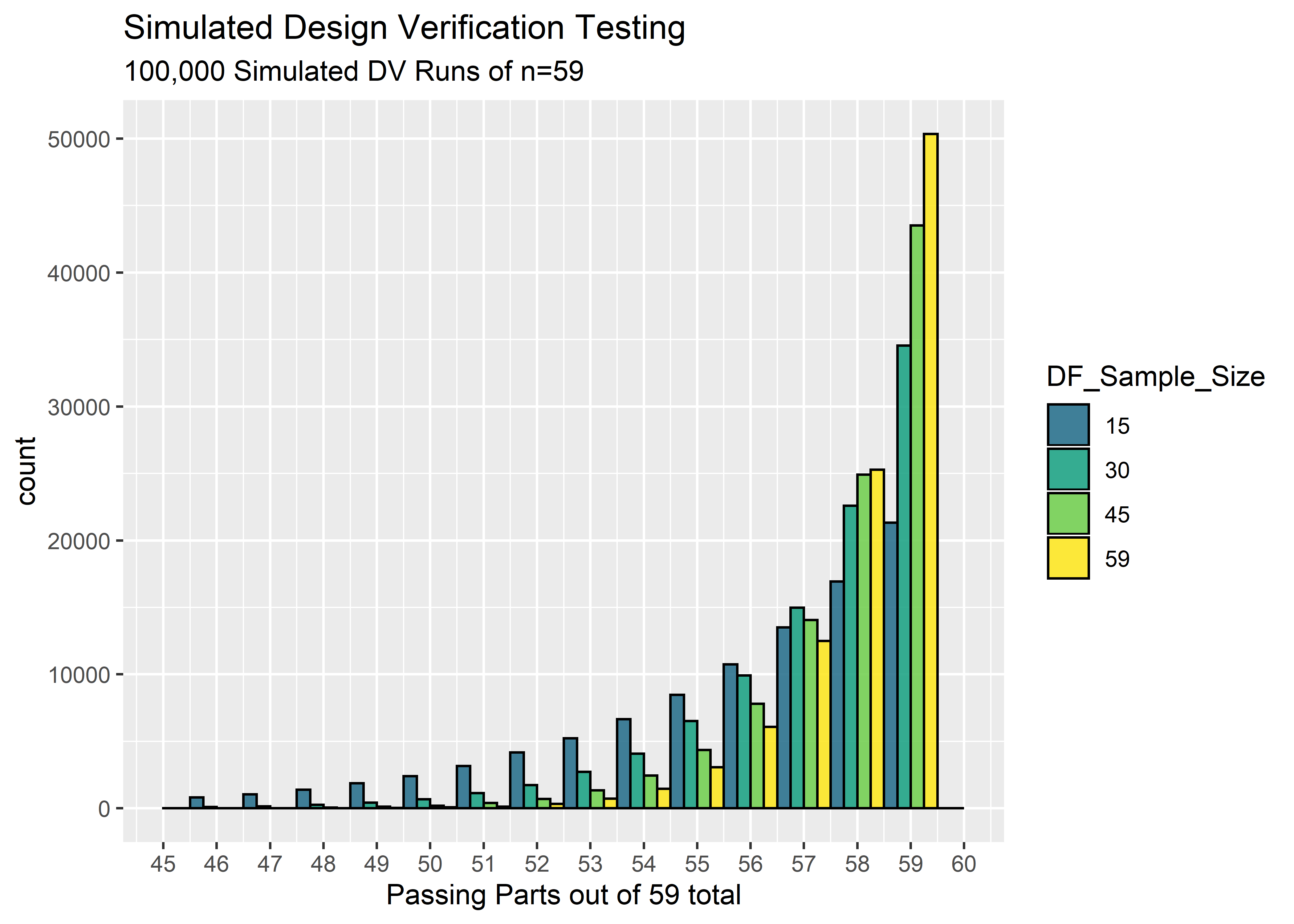
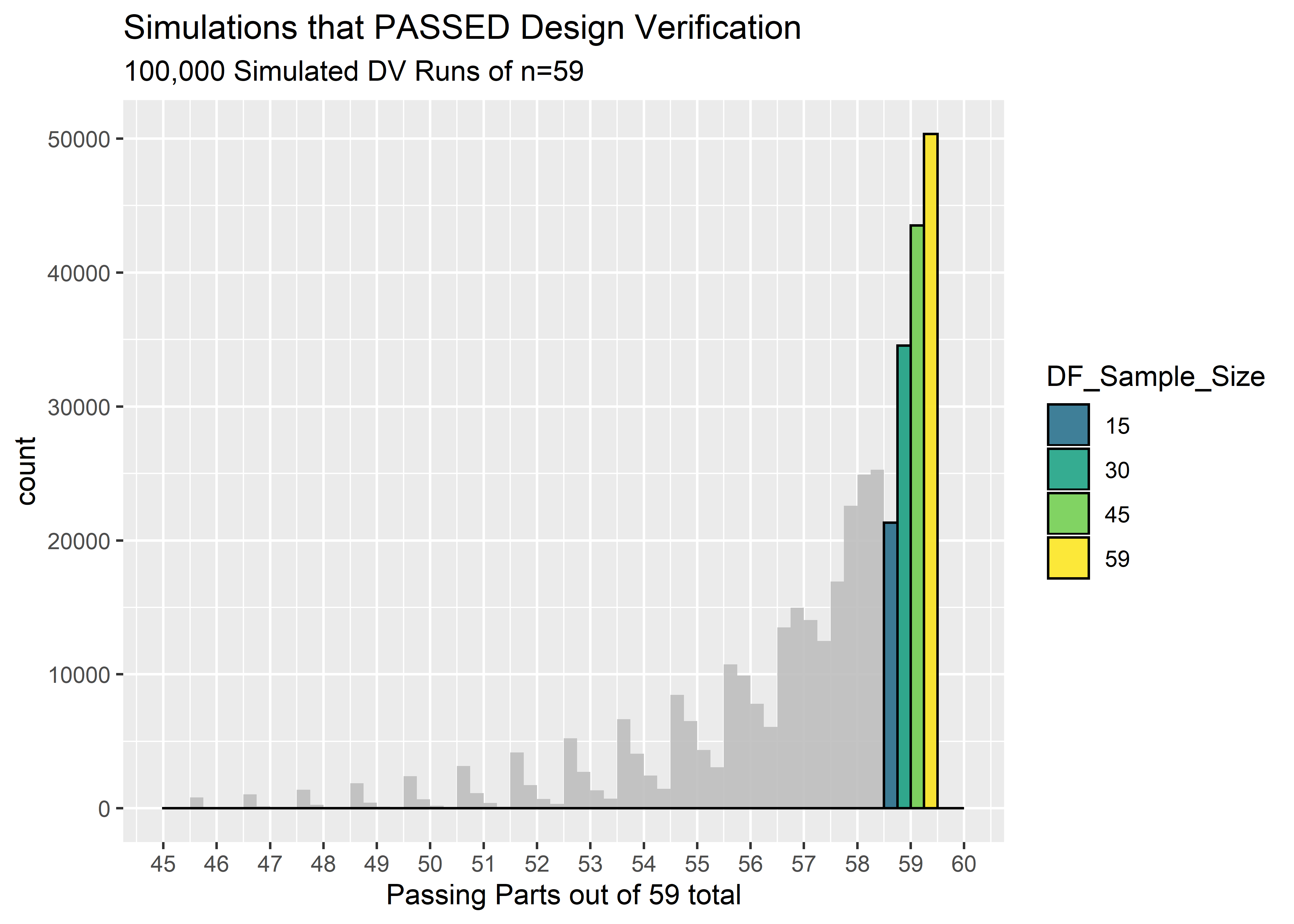
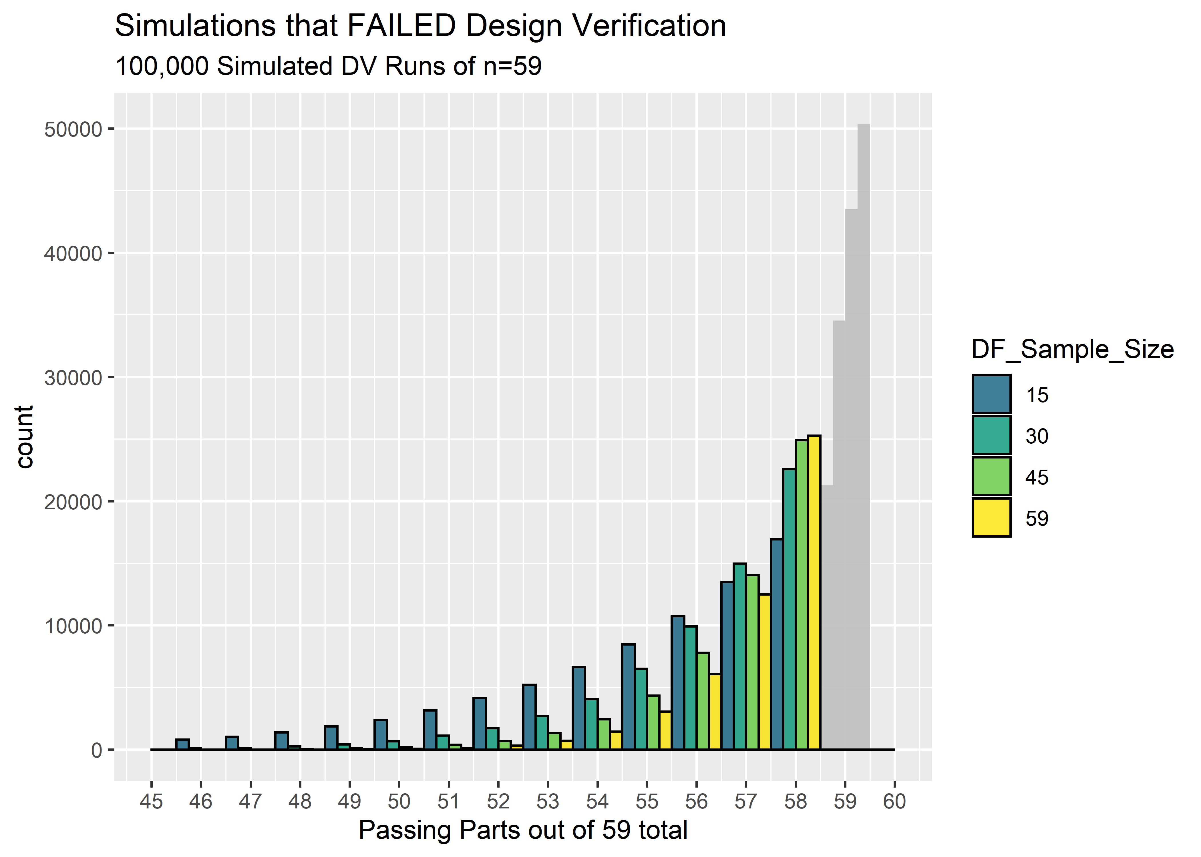
Taking into consideration the uncertainty of the true reliability after the DF testing, the percentage of times we expect to pass Design Verification is shown below. These percentages are calculated as the number of simulated DV runs that achieved 59/59 passing units divided by the total number of simulated DV runs. Any simulation with 58 or less passing units would have failed DV.
\[\mbox{expected probability of passing DV = (number of sims with n=59 pass) / (total sims) }\]
#Function to calculate how many DV simulations resulted in 59/59 passing units
pct_pass_fct <- function(tbl, n){
    pct_dv_pass <- tbl %>% filter(value == 59) %>% nrow() / n_draws
paste("DF with n = ",n, "(all pass): ", pct_dv_pass %>% scales::percent(), "expected probability of next 59/59 passing DV")}| DF with n = 15 (all pass): 21.3% expected probability of next 59/59 passing DV |
| DF with n = 30 (all pass): 34.5% expected probability of next 59/59 passing DV |
| DF with n = 45 (all pass): 43.5% expected probability of next 59/59 passing DV |
| DF with n = 59 (all pass): 50.3% expected probability of next 59/59 passing DV |
The percentage of time we expect to pass Design Verification is shockingly low! Even when we did a full n=59 in Design Freeze, we still only be able to predict 50% success in DV! This is because even with 59/59 passes, we still must account for the possibility that the reliability isn’t 100%. We don’t have enough DF data to shift the credibility all the way near 100%, and when the credibility is spread to include possible reliabilities in the mid .90’s we should always be prepared for the possibility of failing Design Verification.
We could just leave it at that but I have found that when discussing risk, stakeholders want more than just an estimation of the rate of bad outcomes. They want a recommendation and a mitigation plan. Here are a few ideas; can you think of any more?
- Maintain multiple design configurations as long as possible (often not feasible, but provides an out if 1 design fails)
- Perform durability testing as “fatigue-to-failure”. In this methodology, the devices are run to failure and the cycles to failure are treated as variable data. By varying the amplitude of the loading cycles, we can force the devices to fail and understand the uncertainty within the failure envelope. 2
- Fold in information from pre-DF testing, predicate testing, etc to inform the prior better. I will look at the sensitivity of the reliability estimations to the prior in a future post.
- Build redundant design cycles into the project schedule to accomodate additional design turns without falling behind the contracted timeline
Thanks for reading!
Kruschke, Doing Bayesian Data Analysis, https://sites.google.com/site/doingbayesiandataanalysis/↩
Fatigue-to Fracture ASTM Standard: https://www.astm.org/Standards/F3211.htm↩